04 — Post-hoc XAI: SHAP & LIME

Explainable Fraud Detection and Investigation Platform
MIA 5100 machine-learning model with an MIA 5126 XAI extension

This notebook applies the post-hoc explanation methods introduced in MIA 5126 — Essential Concepts in Data Science to the frozen fraud model developed in the first three project notebooks. It adds global and local transparency without retraining the model or changing its operating threshold.

Deliverables

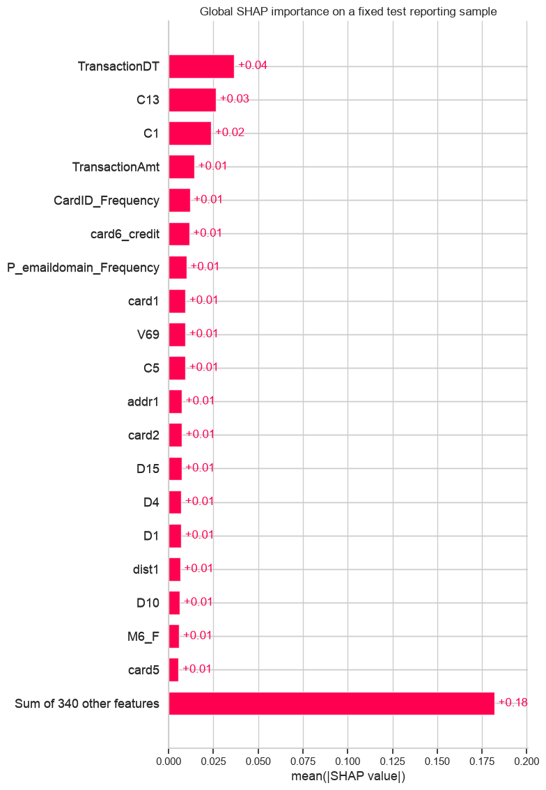
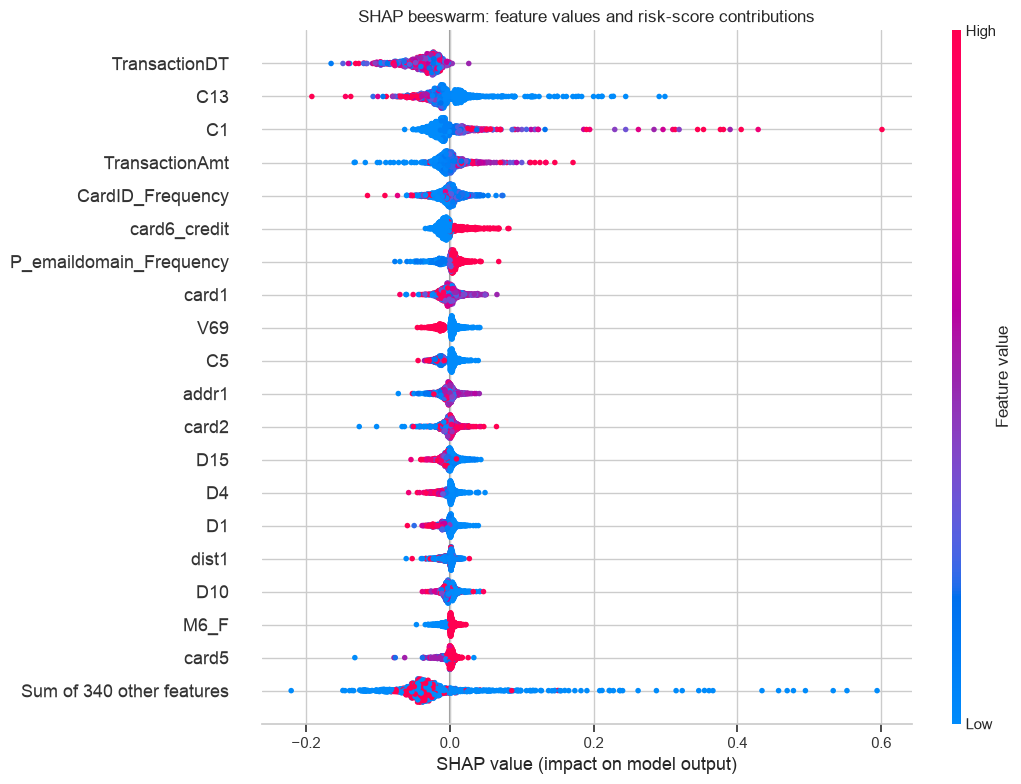
  • Global SHAP bar and beeswarm plots
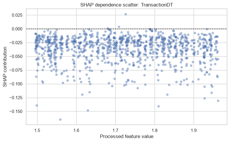
  • SHAP dependence scatter plots
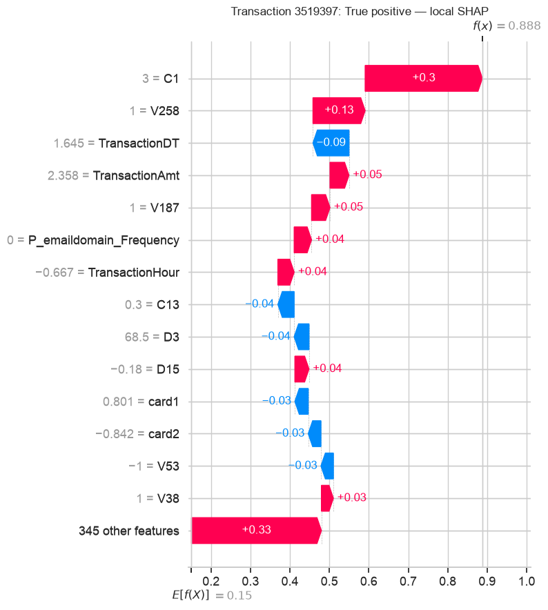
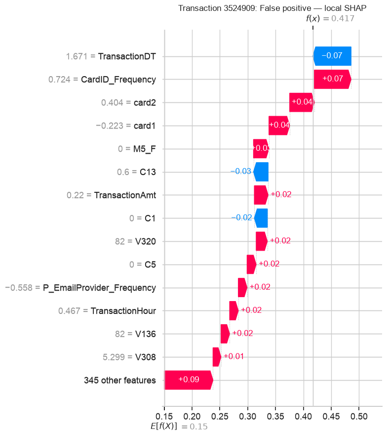
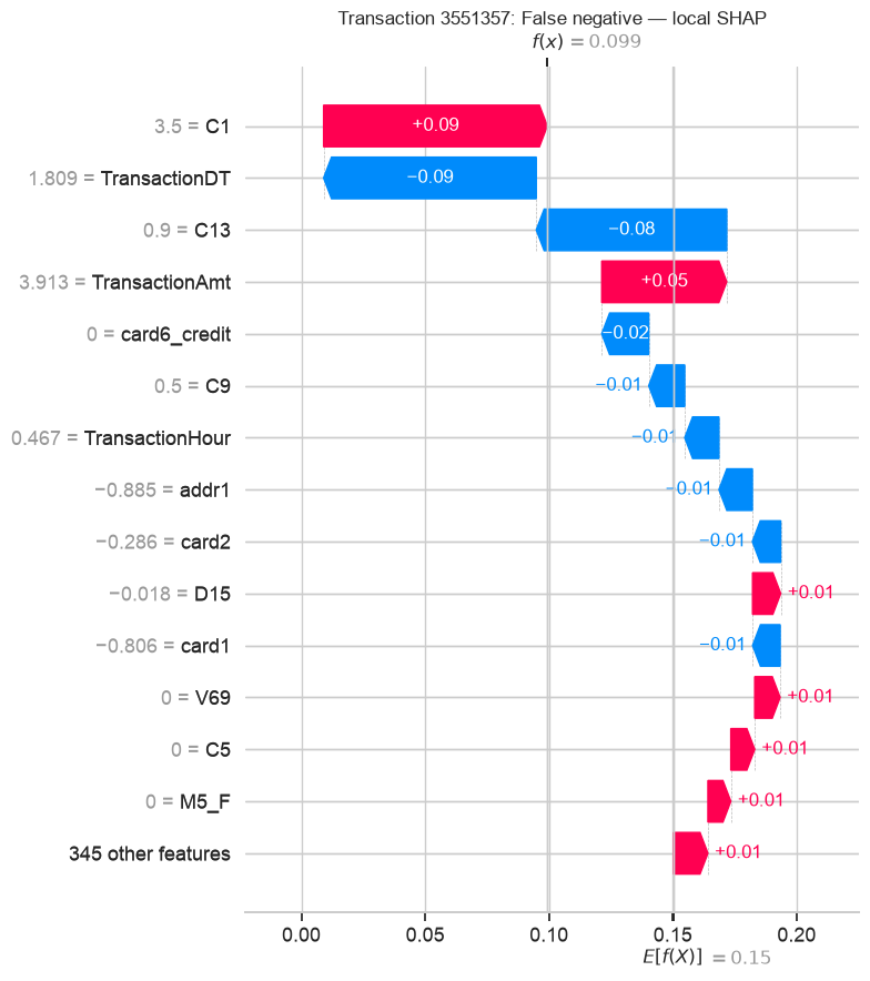
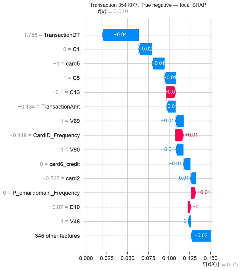
  • Local SHAP waterfall explanations for representative TP, FP, FN, and TN cases
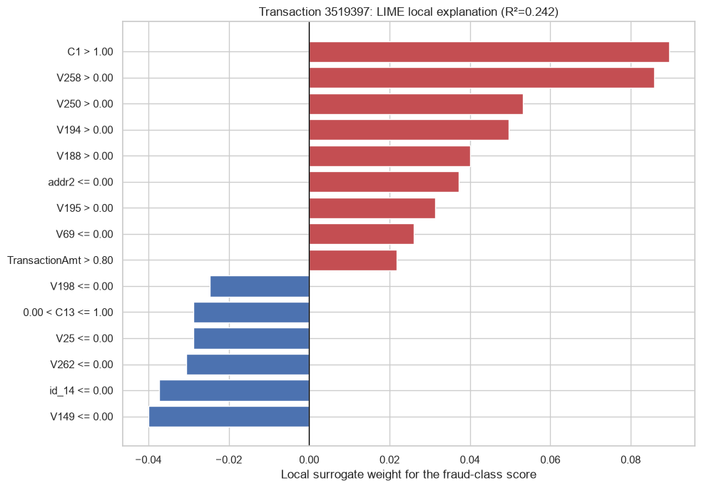
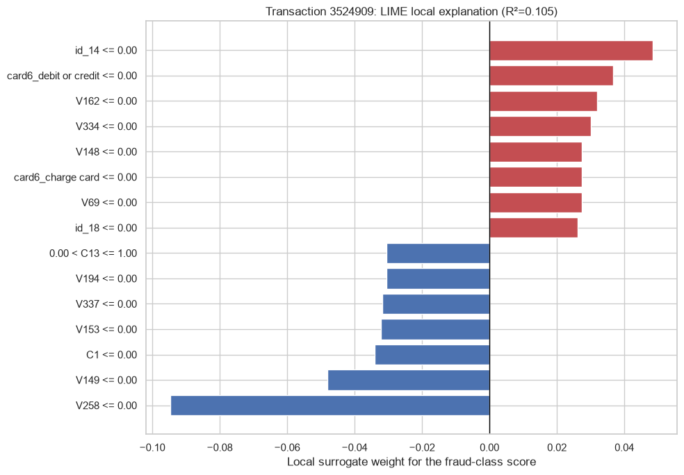
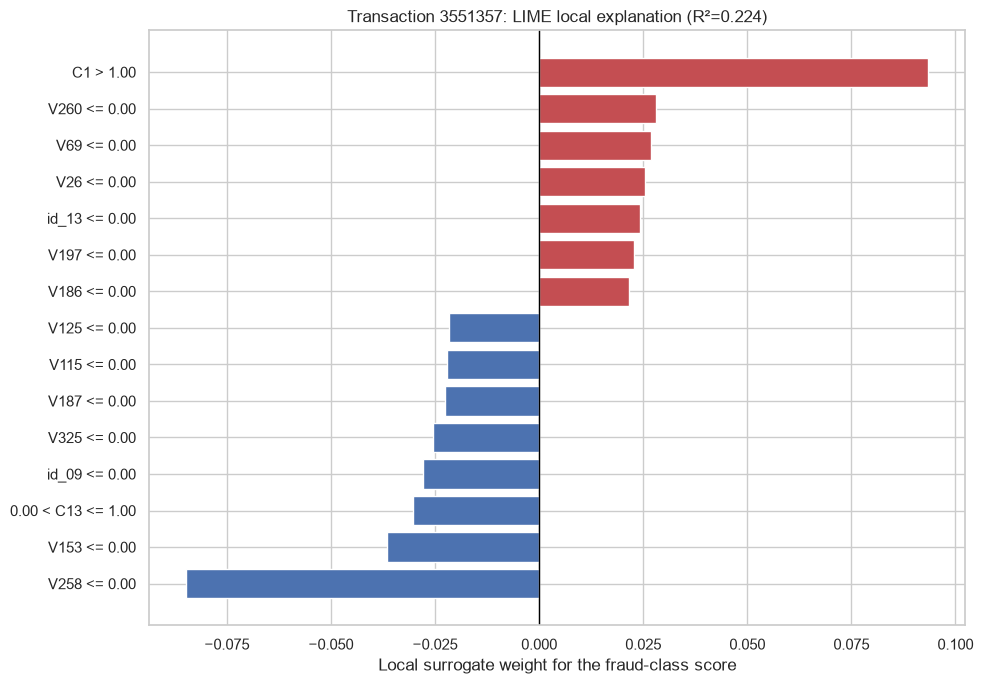
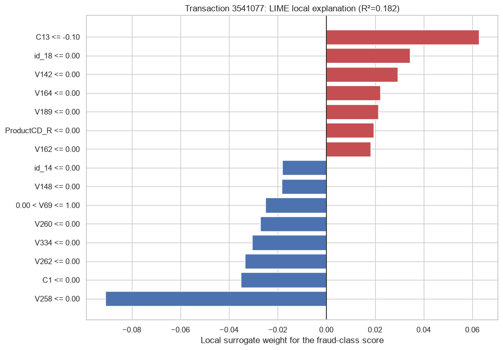
  • LIME explanations for the same cases
  • SHAP/LIME comparison with local-fidelity diagnostics
  • Machine-readable XAI artifacts for the FastAPI and Streamlit applications
  • Explicit explanation limitations and human-review boundaries

Experimental discipline: The champion model, preprocessing schema, and threshold are already frozen. SHAP and LIME are used only for post-hoc reporting. No explanation in this notebook may be used to select features, retrain a model, alter hyperparameters, or change the threshold using final-test information.

Interpretation boundary: A contribution describes how the frozen model behaves for the supplied processed features. It is not evidence that a feature caused fraud, and it does not prove that a transaction is fraudulent or legitimate.

Code
from pathlib import Path
from importlib.metadata import version
from IPython.display import Markdown, display

import json
import os
import platform
import re
import time
import warnings

os.environ.setdefault("MPLCONFIGDIR", "/tmp/matplotlib-cache")

import joblib
import matplotlib.pyplot as plt
import numpy as np
import pandas as pd
import seaborn as sns
import shap

from lime.lime_tabular import LimeTabularExplainer
from scipy.stats import spearmanr

warnings.filterwarnings("ignore", category=FutureWarning)
sns.set_theme(style="whitegrid", context="notebook")
pd.set_option("display.max_columns", 80)
pd.set_option("display.max_colwidth", 120)

RANDOM_STATE = 42
SHAP_BACKGROUND_ROWS = 100
SHAP_GLOBAL_ROWS = 1_000
LIME_REFERENCE_ROWS = 10_000
LIME_NUM_SAMPLES = 5_000
LOCAL_TOP_FEATURES = 20
DISPLAY_TOP_FEATURES = 15

print(f"Python: {platform.python_version()}")
print(f"pandas: {pd.__version__}")
print(f"SHAP: {shap.__version__}")
print(f"LIME: {version('lime')}")
Python: 3.14.6
pandas: 3.0.3
SHAP: 0.51.0
LIME: 0.2.0.1
Code
def find_project_root(start=None):
    candidate = Path(start or Path.cwd()).resolve()
    for parent in [candidate, *candidate.parents]:
        if (parent / "notebooks").exists() and (parent / "models").exists():
            return parent
    raise FileNotFoundError("Could not locate the project repository.")


PROJECT_ROOT = find_project_root()
PROCESSED_PATH = PROJECT_ROOT / "data" / "processed"
TRAINED_MODEL_PATH = PROJECT_ROOT / "models" / "trained"
MODEL_RESULTS_PATH = PROJECT_ROOT / "results" / "model_comparison"
XAI_RESULTS_PATH = PROJECT_ROOT / "results" / "xai"
XAI_FIGURES_PATH = XAI_RESULTS_PATH / "figures"
REPORTS_PATH = PROJECT_ROOT / "reports"

for path in [XAI_RESULTS_PATH, XAI_FIGURES_PATH, REPORTS_PATH]:
    path.mkdir(parents=True, exist_ok=True)

print(f"Project root: {PROJECT_ROOT}")
print(f"XAI output path: {XAI_RESULTS_PATH}")
Project root: /Users/hshazel/Projects/explainable-fraud-investigation-platform
XAI output path: /Users/hshazel/Projects/explainable-fraud-investigation-platform/results/xai

1. Load the frozen model and processed reporting data

The notebook loads the saved champion manifest rather than selecting a model again. The processed test matrix is used only for final post-hoc reporting, while a fixed sample of training rows supplies the SHAP background and LIME reference distribution.

Code
manifest = json.loads(
    (TRAINED_MODEL_PATH / "champion_manifest.json").read_text(encoding="utf-8")
)
model = joblib.load(TRAINED_MODEL_PATH / manifest["model_file"])
model_metadata = json.loads(
    (TRAINED_MODEL_PATH / manifest["metadata_file"]).read_text(encoding="utf-8")
)

X_train = pd.read_parquet(PROCESSED_PATH / "X_train.parquet")
X_test = pd.read_parquet(PROCESSED_PATH / "X_test.parquet")
y_test = pd.read_parquet(PROCESSED_PATH / "y_test.parquet")["isFraud"].reset_index(drop=True)
id_test = pd.read_parquet(PROCESSED_PATH / "id_test.parquet")["TransactionID"].reset_index(drop=True)

threshold = float(model_metadata["decision_threshold"])
feature_names = list(model.feature_names_in_)

predictions = pd.read_parquet(MODEL_RESULTS_PATH / "champion_predictions.parquet")
test_predictions = predictions.loc[predictions["split"] == "test"].copy()
conditions = [
    (test_predictions["isFraud"] == 1) & (test_predictions["predicted_fraud"] == 1),
    (test_predictions["isFraud"] == 0) & (test_predictions["predicted_fraud"] == 1),
    (test_predictions["isFraud"] == 1) & (test_predictions["predicted_fraud"] == 0),
]
test_predictions["Outcome"] = np.select(
    conditions,
    ["True positive", "False positive", "False negative"],
    default="True negative",
)


def select_representative_case(frame, outcome):
    subset = frame.loc[frame["Outcome"] == outcome].copy()
    median_score = subset["fraud_risk_score"].median()
    subset["Distance to outcome median"] = (
        subset["fraud_risk_score"] - median_score
    ).abs()
    return subset.sort_values(
        ["Distance to outcome median", "TransactionID"]
    ).iloc[0]


outcome_order = ["True positive", "False positive", "False negative", "True negative"]
selected_cases = pd.DataFrame([
    select_representative_case(test_predictions, outcome)
    for outcome in outcome_order
])


def feature_family(feature):
    if feature in {"TransactionDT", "TransactionAmt", "TransactionHour", "TransactionDay"}:
        return "Transaction"
    if feature.startswith("card") or "CardID" in feature:
        return "Card"
    if feature.startswith("addr") or feature.startswith("dist"):
        return "Address / distance"
    if re.fullmatch(r"C\d+", feature):
        return "Count (C)"
    if re.fullmatch(r"D\d+", feature):
        return "Time delta (D)"
    if re.fullmatch(r"M\d+.*", feature):
        return "Match flag (M)"
    if re.fullmatch(r"V\d+", feature):
        return "Anonymous V"
    if feature.startswith("id_"):
        return "Identity"
    if "email" in feature.lower():
        return "Email"
    if "device" in feature.lower():
        return "Device"
    if feature.startswith("ProductCD"):
        return "Product"
    return "Engineered / other"


gain_scores = model.get_booster().get_score(importance_type="gain")
native_importance = pd.DataFrame({"Feature": feature_names})
native_importance["Gain"] = native_importance["Feature"].map(gain_scores).fillna(0.0)
native_importance["Normalized Gain"] = (
    native_importance["Gain"] / native_importance["Gain"].sum()
)
native_importance = native_importance.sort_values(
    "Normalized Gain", ascending=False
).reset_index(drop=True)
native_importance["Gain Rank"] = np.arange(1, len(native_importance) + 1)
native_importance["Feature family"] = native_importance["Feature"].map(feature_family)

assert manifest["model_name"] == "XGBoost (tuned)"
assert X_train.columns.tolist() == feature_names
assert X_test.columns.tolist() == feature_names
assert len(feature_names) == int(model_metadata["feature_count"]) == 359
assert len(X_test) == len(y_test) == len(id_test)
assert id_test.is_unique
assert set(selected_cases["TransactionID"]).issubset(set(id_test))

display(Markdown(
    f"**Frozen champion:** {manifest['model_name']}  \n"
    f"**Decision threshold:** {threshold:.6f}  \n"
    f"**Processed features:** {len(feature_names):,}  \n"
    f"**Test rows available for reporting:** {len(X_test):,}"
))

Frozen champion: XGBoost (tuned)
Decision threshold: 0.275698
Processed features: 359
Test rows available for reporting: 88,581

Code
id_to_position = pd.Series(
    np.arange(len(id_test), dtype="int64"), index=id_test.to_numpy()
)
selected_case_ids = selected_cases["TransactionID"].astype("int64").tolist()
local_positions = [int(id_to_position.loc[transaction_id]) for transaction_id in selected_case_ids]
local_features = X_test.iloc[local_positions].reset_index(drop=True)

saved_scores = selected_cases.set_index("TransactionID").loc[
    selected_case_ids, "fraud_risk_score"
].to_numpy()
recomputed_scores = model.predict_proba(local_features)[:, 1]
np.testing.assert_allclose(recomputed_scores, saved_scores, rtol=1e-5, atol=1e-6)

case_context = selected_cases.set_index("TransactionID").loc[
    selected_case_ids,
    ["Outcome", "fraud_risk_score", "predicted_fraud", "isFraud"],
].reset_index()
display(case_context.style.format({
    "fraud_risk_score": "{:.4f}",
}))
print("Representative case scores match the frozen predictions from 03_model_selection_and_evaluation.ipynb.")
  TransactionID Outcome fraud_risk_score predicted_fraud isFraud
0 3519397 True positive 0.8880 1 1
1 3524909 False positive 0.4169 1 0
2 3551357 False negative 0.0993 0 1
3 3541077 True negative 0.0192 0 0
Representative case scores match the frozen predictions from 03_model_selection_and_evaluation.ipynb.

2. Fixed explanation samples

  • SHAP background: 100 training rows, consistent with the documented 100–1,000 row interventional background guidance.
  • Global SHAP reporting sample: 1,000 randomly selected test rows. This is a reproducible approximation of global behavior, not a new evaluation sample.
  • Local cases: One median-risk test case from each confusion-matrix outcome (true positive, false positive, false negative, and true negative), selected deterministically from 03_model_selection_and_evaluation.ipynb predictions.
  • LIME reference: 10,000 training rows to estimate perturbation distributions without densifying all 413,378 training observations.
Code
rng = np.random.default_rng(RANDOM_STATE)
background_positions = np.sort(
    rng.choice(len(X_train), size=SHAP_BACKGROUND_ROWS, replace=False)
)
global_positions = np.sort(
    rng.choice(len(X_test), size=SHAP_GLOBAL_ROWS, replace=False)
)

shap_background = X_train.iloc[background_positions].copy()
global_features = X_test.iloc[global_positions].copy()
global_ids = id_test.iloc[global_positions].reset_index(drop=True)
global_labels = y_test.iloc[global_positions].reset_index(drop=True)

sample_manifest = pd.DataFrame({
    "TransactionID": global_ids,
    "isFraud": global_labels.astype("int8"),
    "TestRowPosition": global_positions,
})

print(f"SHAP background rows: {len(shap_background):,}")
print(f"Global SHAP reporting rows: {len(global_features):,}")
print(f"Global sample fraud rate: {global_labels.mean():.2%}")
print(f"Local representative cases: {len(local_features):,}")
SHAP background rows: 100
Global SHAP reporting rows: 1,000
Global sample fraud rate: 3.70%
Local representative cases: 4

3. Tree SHAP in model-score space

TreeExplainer is model-specific and efficient for the XGBoost champion. The explainer uses an interventional training background and model_output="probability", so the base value plus feature contributions reconstructs the model’s predict_proba class-1 output.

The output is still described as an uncalibrated fraud risk score, consistent with 03_model_selection_and_evaluation.ipynb. It must not be interpreted as an empirically calibrated probability of fraud.

Code
shap_start = time.time()
tree_explainer = shap.TreeExplainer(
    model,
    data=shap_background,
    feature_perturbation="interventional",
    model_output="probability",
)
global_shap = tree_explainer(global_features, check_additivity=False)
local_shap = tree_explainer(local_features, check_additivity=False)
shap_seconds = time.time() - shap_start


def reconstructed_output(explanation):
    base = np.asarray(explanation.base_values, dtype=float)
    if base.ndim == 0:
        base = np.repeat(base, len(explanation.values))
    return base + np.asarray(explanation.values).sum(axis=1)


global_reconstructed = reconstructed_output(global_shap)
local_reconstructed = reconstructed_output(local_shap)
global_model_scores = model.predict_proba(global_features)[:, 1]
local_model_scores = model.predict_proba(local_features)[:, 1]

global_reconstruction_error = float(
    np.max(np.abs(global_reconstructed - global_model_scores))
)
local_reconstruction_error = float(
    np.max(np.abs(local_reconstructed - local_model_scores))
)

assert global_shap.shape == global_features.shape
assert local_shap.shape == local_features.shape
assert global_reconstruction_error < 1e-5
assert local_reconstruction_error < 1e-5

print(f"SHAP computation time: {shap_seconds:.2f} seconds")
print(f"Maximum global reconstruction error: {global_reconstruction_error:.2e}")
print(f"Maximum local reconstruction error: {local_reconstruction_error:.2e}")
print(f"SHAP base risk score: {float(np.asarray(global_shap.base_values)[0]):.4f}")

 64%|=============       | 637/1000 [00:11<00:06]       
 70%|==============      | 698/1000 [00:12<00:05]       
 76%|===============     | 760/1000 [00:13<00:04]       
 82%|================    | 822/1000 [00:14<00:03]       
 88%|==================  | 885/1000 [00:15<00:01]       
 95%|=================== | 946/1000 [00:16<00:00]       
SHAP computation time: 16.44 seconds
Maximum global reconstruction error: 3.82e-07
Maximum local reconstruction error: 1.53e-07
SHAP base risk score: 0.1504

4. Global SHAP explanations

Code
global_importance = pd.DataFrame({
    "Feature": feature_names,
    "Mean absolute SHAP": np.abs(global_shap.values).mean(axis=0),
    "Mean signed SHAP": global_shap.values.mean(axis=0),
    "Positive contribution share": (global_shap.values > 0).mean(axis=0),
}).sort_values("Mean absolute SHAP", ascending=False).reset_index(drop=True)

global_importance["SHAP rank"] = np.arange(1, len(global_importance) + 1)
total_shap = global_importance["Mean absolute SHAP"].sum()
global_importance["Normalized mean absolute SHAP"] = (
    global_importance["Mean absolute SHAP"] / total_shap
)

native_columns = native_importance[[
    "Feature", "Normalized Gain", "Gain Rank", "Feature family"
]].copy()
global_importance = global_importance.merge(
    native_columns, on="Feature", how="left", validate="one_to_one"
)

display(global_importance.head(20).style.format({
    "Mean absolute SHAP": "{:.5f}",
    "Mean signed SHAP": "{:+.5f}",
    "Positive contribution share": "{:.1%}",
    "Normalized mean absolute SHAP": "{:.2%}",
    "Normalized Gain": "{:.2%}",
}))
  Feature Mean absolute SHAP Mean signed SHAP Positive contribution share SHAP rank Normalized mean absolute SHAP Normalized Gain Gain Rank Feature family
0 TransactionDT 0.03664 -0.03658 0.3% 1 9.06% 0.20% 127 Transaction
1 C13 0.02640 -0.00288 34.9% 2 6.53% 0.54% 19 Count (C)
2 C1 0.02375 +0.00253 31.9% 3 5.87% 0.55% 18 Count (C)
3 TransactionAmt 0.01434 +0.00024 43.6% 4 3.55% 0.21% 104 Transaction
4 CardID_Frequency 0.01184 -0.00253 45.9% 5 2.93% 0.22% 99 Card
5 card6_credit 0.01147 -0.00112 29.2% 6 2.84% 0.73% 11 Card
6 P_emaildomain_Frequency 0.00999 +0.00072 69.7% 7 2.47% 0.23% 91 Email
7 card1 0.00937 -0.00103 44.2% 8 2.32% 0.19% 138 Card
8 V69 0.00932 -0.00123 64.3% 9 2.31% 4.73% 2 Anonymous V
9 C5 0.00931 -0.00207 60.8% 10 2.30% 0.67% 13 Count (C)
10 addr1 0.00736 -0.00268 39.4% 11 1.82% 0.19% 150 Address / distance
11 card2 0.00735 -0.00110 47.4% 12 1.82% 0.19% 149 Card
12 D15 0.00715 -0.00041 47.6% 13 1.77% 0.21% 110 Time delta (D)
13 D4 0.00702 -0.00192 54.2% 14 1.74% 0.20% 126 Time delta (D)
14 D1 0.00693 -0.00201 50.9% 15 1.71% 0.22% 95 Time delta (D)
15 dist1 0.00647 -0.00210 57.9% 16 1.60% 0.19% 152 Address / distance
16 D10 0.00626 -0.00031 44.3% 17 1.55% 0.22% 97 Time delta (D)
17 M6_F 0.00584 -0.00105 64.0% 18 1.44% 0.28% 53 Match flag (M)
18 card5 0.00555 -0.00126 60.0% 19 1.37% 0.21% 108 Card
19 V90 0.00537 -0.00126 62.6% 20 1.33% 1.65% 5 Anonymous V
Code
shap.plots.bar(global_shap, max_display=20, show=False)
plt.title("Global SHAP importance on a fixed test reporting sample")
plt.tight_layout()
global_bar_file = XAI_FIGURES_PATH / "shap_global_bar.png"
plt.savefig(global_bar_file, dpi=180, bbox_inches="tight")
plt.show()

shap.plots.beeswarm(
    global_shap,
    max_display=20,
    show=False,
    plot_size=(11, 8),
)
plt.title("SHAP beeswarm: feature values and risk-score contributions")
plt.tight_layout()
global_beeswarm_file = XAI_FIGURES_PATH / "shap_global_beeswarm.png"
plt.savefig(global_beeswarm_file, dpi=180, bbox_inches="tight")
plt.show()

print(f"Saved: {global_bar_file.name}, {global_beeswarm_file.name}")

Saved: shap_global_bar.png, shap_global_beeswarm.png

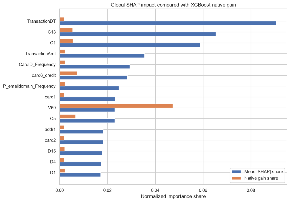
SHAP versus XGBoost native gain

Native gain measures training-time split improvement. Mean absolute SHAP measures average prediction impact on the fixed reporting sample. Agreement is useful context, but the rankings are not expected to be identical because they answer different questions.

Code
rank_correlation = spearmanr(
    global_importance["SHAP rank"],
    global_importance["Gain Rank"],
    nan_policy="omit",
)
spearman_rank_correlation = float(rank_correlation.statistic)

comparison_features = global_importance.head(15).copy().sort_values(
    "Normalized mean absolute SHAP"
)
positions = np.arange(len(comparison_features))
height = 0.38

fig, ax = plt.subplots(figsize=(10, 7))
ax.barh(
    positions - height / 2,
    comparison_features["Normalized mean absolute SHAP"],
    height,
    label="Mean |SHAP| share",
)
ax.barh(
    positions + height / 2,
    comparison_features["Normalized Gain"],
    height,
    label="Native gain share",
)
ax.set_yticks(positions, comparison_features["Feature"])
ax.set_xlabel("Normalized importance share")
ax.set_title("Global SHAP impact compared with XGBoost native gain")
ax.legend()
plt.tight_layout()
importance_comparison_file = XAI_FIGURES_PATH / "shap_vs_native_importance.png"
plt.savefig(importance_comparison_file, dpi=180, bbox_inches="tight")
plt.show()

print(f"Spearman rank correlation across features: {spearman_rank_correlation:.3f}")

Spearman rank correlation across features: 0.621

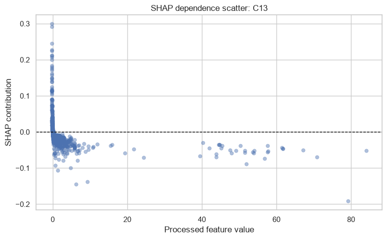
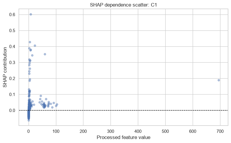
SHAP dependence scatter plots

Each plot relates a processed feature value to that feature’s SHAP contribution across the fixed reporting sample. The vertical axis is the change in the model’s uncalibrated risk score relative to the background expectation. Patterns are associative descriptions of model behavior, not causal effects.

Code
dependence_features = global_importance.head(3)["Feature"].tolist()
dependence_figure_files = {}

for feature in dependence_features:
    feature_index = feature_names.index(feature)
    plot_data = pd.DataFrame({
        "Processed feature value": global_features[feature].to_numpy(),
        "SHAP contribution": global_shap.values[:, feature_index],
    })
    fig, ax = plt.subplots(figsize=(8, 5))
    sns.scatterplot(
        data=plot_data,
        x="Processed feature value",
        y="SHAP contribution",
        alpha=0.45,
        s=28,
        edgecolor=None,
        ax=ax,
    )
    ax.axhline(0, color="black", linewidth=1, linestyle="--")
    ax.set_title(f"SHAP dependence scatter: {feature}")
    plt.tight_layout()
    safe_name = re.sub(r"[^A-Za-z0-9_-]+", "_", feature)
    figure_file = XAI_FIGURES_PATH / f"shap_dependence_{safe_name}.png"
    plt.savefig(figure_file, dpi=180, bbox_inches="tight")
    plt.show()
    dependence_figure_files[feature] = figure_file.name

print(f"Dependence features: {dependence_features}")

Dependence features: ['TransactionDT', 'C13', 'C1']

5. Local SHAP waterfall explanations

Code
local_shap_records = []
shap_waterfall_files = {}

for case_index, transaction_id in enumerate(selected_case_ids):
    context = case_context.loc[
        case_context["TransactionID"] == transaction_id
    ].iloc[0]
    values = np.asarray(local_shap.values[case_index])
    absolute_order = np.argsort(np.abs(values))[::-1]

    for rank, feature_index in enumerate(absolute_order, start=1):
        contribution = float(values[feature_index])
        local_shap_records.append({
            "TransactionID": int(transaction_id),
            "Feature": feature_names[feature_index],
            "Processed feature value": float(local_features.iloc[case_index, feature_index]),
            "SHAP contribution": contribution,
            "Absolute SHAP contribution": abs(contribution),
            "Direction": (
                "Higher risk score" if contribution > 0
                else "Lower risk score" if contribution < 0
                else "Neutral"
            ),
            "Rank": rank,
            "Base risk score": float(np.asarray(local_shap.base_values)[case_index]),
            "Model risk score": float(local_model_scores[case_index]),
            "Decision threshold": threshold,
        })

    shap.plots.waterfall(
        local_shap[case_index],
        max_display=DISPLAY_TOP_FEATURES,
        show=False,
    )
    plt.title(
        f"Transaction {transaction_id}: {context['Outcome']} — local SHAP"
    )
    plt.tight_layout()
    figure_file = XAI_FIGURES_PATH / f"shap_waterfall_{transaction_id}.png"
    plt.savefig(figure_file, dpi=180, bbox_inches="tight")
    plt.show()
    shap_waterfall_files[str(transaction_id)] = figure_file.name

local_shap_table = pd.DataFrame(local_shap_records)
display(
    local_shap_table.query("Rank <= 10").style.format({
        "Processed feature value": "{:.4f}",
        "SHAP contribution": "{:+.5f}",
        "Absolute SHAP contribution": "{:.5f}",
        "Base risk score": "{:.4f}",
        "Model risk score": "{:.4f}",
        "Decision threshold": "{:.4f}",
    })
)

  TransactionID Feature Processed feature value SHAP contribution Absolute SHAP contribution Direction Rank Base risk score Model risk score Decision threshold
0 3519397 C1 3.0000 +0.29729 0.29729 Higher risk score 1 0.1504 0.8880 0.2757
1 3519397 V258 1.0000 +0.13230 0.13230 Higher risk score 2 0.1504 0.8880 0.2757
2 3519397 TransactionDT 1.6452 -0.09135 0.09135 Lower risk score 3 0.1504 0.8880 0.2757
3 3519397 TransactionAmt 2.3577 +0.04814 0.04814 Higher risk score 4 0.1504 0.8880 0.2757
4 3519397 V187 1.0000 +0.04677 0.04677 Higher risk score 5 0.1504 0.8880 0.2757
5 3519397 P_emaildomain_Frequency 0.0000 +0.04410 0.04410 Higher risk score 6 0.1504 0.8880 0.2757
6 3519397 TransactionHour -0.6667 +0.04130 0.04130 Higher risk score 7 0.1504 0.8880 0.2757
7 3519397 C13 0.3000 -0.04122 0.04122 Lower risk score 8 0.1504 0.8880 0.2757
8 3519397 D3 68.5000 -0.03771 0.03771 Lower risk score 9 0.1504 0.8880 0.2757
9 3519397 D15 -0.1798 +0.03583 0.03583 Higher risk score 10 0.1504 0.8880 0.2757
359 3524909 TransactionDT 1.6714 -0.06871 0.06871 Lower risk score 1 0.1504 0.4169 0.2757
360 3524909 CardID_Frequency 0.7245 +0.06596 0.06596 Higher risk score 2 0.1504 0.4169 0.2757
361 3524909 card2 0.4040 +0.04431 0.04431 Higher risk score 3 0.1504 0.4169 0.2757
362 3524909 card1 -0.2226 +0.03718 0.03718 Higher risk score 4 0.1504 0.4169 0.2757
363 3524909 M5_F 0.0000 +0.02775 0.02775 Higher risk score 5 0.1504 0.4169 0.2757
364 3524909 C13 0.6000 -0.02625 0.02625 Lower risk score 6 0.1504 0.4169 0.2757
365 3524909 TransactionAmt 0.2200 +0.02474 0.02474 Higher risk score 7 0.1504 0.4169 0.2757
366 3524909 C1 0.0000 -0.02335 0.02335 Lower risk score 8 0.1504 0.4169 0.2757
367 3524909 V320 82.0000 +0.02005 0.02005 Higher risk score 9 0.1504 0.4169 0.2757
368 3524909 C5 0.0000 +0.01635 0.01635 Higher risk score 10 0.1504 0.4169 0.2757
718 3551357 C1 3.5000 +0.09034 0.09034 Higher risk score 1 0.1504 0.0993 0.2757
719 3551357 TransactionDT 1.8093 -0.08587 0.08587 Lower risk score 2 0.1504 0.0993 0.2757
720 3551357 C13 0.9000 -0.07691 0.07691 Lower risk score 3 0.1504 0.0993 0.2757
721 3551357 TransactionAmt 3.9129 +0.05047 0.05047 Higher risk score 4 0.1504 0.0993 0.2757
722 3551357 card6_credit 0.0000 -0.01896 0.01896 Lower risk score 5 0.1504 0.0993 0.2757
723 3551357 C9 0.5000 -0.01455 0.01455 Lower risk score 6 0.1504 0.0993 0.2757
724 3551357 TransactionHour 0.4667 -0.01381 0.01381 Lower risk score 7 0.1504 0.0993 0.2757
725 3551357 addr1 -0.8852 -0.01350 0.01350 Lower risk score 8 0.1504 0.0993 0.2757
726 3551357 card2 -0.2862 -0.01145 0.01145 Lower risk score 9 0.1504 0.0993 0.2757
727 3551357 D15 -0.0175 +0.01137 0.01137 Higher risk score 10 0.1504 0.0993 0.2757
1077 3541077 TransactionDT 1.7577 -0.04406 0.04406 Lower risk score 1 0.1504 0.0192 0.2757
1078 3541077 C1 0.0000 -0.01610 0.01610 Lower risk score 2 0.1504 0.0192 0.2757
1079 3541077 card5 -1.0000 -0.01488 0.01488 Lower risk score 3 0.1504 0.0192 0.2757
1080 3541077 C5 1.0000 -0.01377 0.01377 Lower risk score 4 0.1504 0.0192 0.2757
1081 3541077 C13 -0.1000 +0.01111 0.01111 Higher risk score 5 0.1504 0.0192 0.2757
1082 3541077 TransactionAmt -0.1341 -0.01062 0.01062 Lower risk score 6 0.1504 0.0192 0.2757
1083 3541077 V69 1.0000 -0.00983 0.00983 Lower risk score 7 0.1504 0.0192 0.2757
1084 3541077 CardID_Frequency -0.1480 +0.00958 0.00958 Higher risk score 8 0.1504 0.0192 0.2757
1085 3541077 V90 1.0000 -0.00920 0.00920 Lower risk score 9 0.1504 0.0192 0.2757
1086 3541077 card6_credit 0.0000 -0.00845 0.00845 Lower risk score 10 0.1504 0.0192 0.2757

6. LIME explanations for the same cases

LIME is model-agnostic. It perturbs a processed transaction and fits a sparse local linear surrogate around that case. The displayed weights describe the surrogate, not XGBoost directly.

The local surrogate’s weighted R² (LIME local fidelity R2) is reported for every case. Low fidelity means the linear approximation does not closely reproduce the nonlinear champion in that neighborhood; its feature weights should then receive limited evidentiary weight.

Code
lime_reference = X_train.sample(
    n=min(LIME_REFERENCE_ROWS, len(X_train)),
    random_state=RANDOM_STATE,
)
lime_explainer = LimeTabularExplainer(
    lime_reference.to_numpy(),
    feature_names=feature_names,
    class_names=["Non-fraud class", "Fraud class"],
    mode="classification",
    discretize_continuous=True,
    random_state=RANDOM_STATE,
)

lime_records = []
lime_case_summary_records = []
lime_figure_files = {}
lime_start = time.time()

for case_index, transaction_id in enumerate(selected_case_ids):
    explanation = lime_explainer.explain_instance(
        local_features.iloc[case_index].to_numpy(),
        model.predict_proba,
        labels=(1,),
        num_features=LOCAL_TOP_FEATURES,
        num_samples=LIME_NUM_SAMPLES,
    )
    map_items = explanation.as_map()[1]
    list_items = explanation.as_list(label=1)

    case_records = []
    for (feature_index, weight), (condition, displayed_weight) in zip(
        map_items, list_items
    ):
        assert np.isclose(weight, displayed_weight)
        record = {
            "TransactionID": int(transaction_id),
            "Feature": feature_names[int(feature_index)],
            "Condition": condition,
            "Processed feature value": float(
                local_features.iloc[case_index, int(feature_index)]
            ),
            "LIME weight": float(weight),
            "Absolute LIME weight": abs(float(weight)),
            "Direction": (
                "Higher risk score" if weight > 0 else "Lower risk score"
            ),
        }
        case_records.append(record)

    case_records = sorted(
        case_records,
        key=lambda record: record["Absolute LIME weight"],
        reverse=True,
    )
    for rank, record in enumerate(case_records, start=1):
        record["Rank"] = rank
        record["LIME local fidelity R2"] = float(explanation.score)
        record["LIME local prediction"] = float(np.ravel(explanation.local_pred)[0])
        record["Model risk score"] = float(local_model_scores[case_index])
        record["Decision threshold"] = threshold
        lime_records.append(record)

    lime_case_summary_records.append({
        "TransactionID": int(transaction_id),
        "LIME local fidelity R2": float(explanation.score),
        "LIME local prediction": float(np.ravel(explanation.local_pred)[0]),
        "Model risk score": float(local_model_scores[case_index]),
        "Absolute local prediction error": abs(
            float(np.ravel(explanation.local_pred)[0])
            - float(local_model_scores[case_index])
        ),
    })

    plot_frame = pd.DataFrame(case_records).head(DISPLAY_TOP_FEATURES)
    plot_frame = plot_frame.sort_values("LIME weight")
    colors = np.where(plot_frame["LIME weight"] >= 0, "#c44e52", "#4c72b0")
    fig, ax = plt.subplots(figsize=(10, 7))
    ax.barh(plot_frame["Condition"], plot_frame["LIME weight"], color=colors)
    ax.axvline(0, color="black", linewidth=1)
    ax.set_xlabel("Local surrogate weight for the fraud-class score")
    ax.set_title(
        f"Transaction {transaction_id}: LIME local explanation "
        f"(R²={explanation.score:.3f})"
    )
    plt.tight_layout()
    figure_file = XAI_FIGURES_PATH / f"lime_{transaction_id}.png"
    plt.savefig(figure_file, dpi=180, bbox_inches="tight")
    plt.show()
    lime_figure_files[str(transaction_id)] = figure_file.name

lime_seconds = time.time() - lime_start
local_lime_table = pd.DataFrame(lime_records)
lime_case_summary = pd.DataFrame(lime_case_summary_records)

display(lime_case_summary.style.format({
    "LIME local fidelity R2": "{:.3f}",
    "LIME local prediction": "{:.4f}",
    "Model risk score": "{:.4f}",
    "Absolute local prediction error": "{:.4f}",
}))
print(f"LIME computation time: {lime_seconds:.2f} seconds")

  TransactionID LIME local fidelity R2 LIME local prediction Model risk score Absolute local prediction error
0 3519397 0.242 0.3961 0.8880 0.4919
1 3524909 0.105 0.0164 0.4169 0.4005
2 3551357 0.224 0.1046 0.0993 0.0052
3 3541077 0.182 0.0498 0.0192 0.0306
LIME computation time: 1.37 seconds

7. SHAP and LIME local comparison

Code
comparison_records = []
comparison_top_k = 10

for transaction_id in selected_case_ids:
    shap_case = local_shap_table.query(
        "TransactionID == @transaction_id and Rank <= @comparison_top_k"
    )
    lime_case = local_lime_table.query(
        "TransactionID == @transaction_id and Rank <= @comparison_top_k"
    )
    shap_features = set(shap_case["Feature"])
    lime_features = set(lime_case["Feature"])
    overlap = shap_features & lime_features
    union = shap_features | lime_features

    shap_sign = shap_case.set_index("Feature")["SHAP contribution"].map(np.sign)
    lime_sign = lime_case.set_index("Feature")["LIME weight"].map(np.sign)
    sign_agreements = [
        shap_sign.loc[feature] == lime_sign.loc[feature]
        for feature in overlap
    ]
    lime_summary = lime_case_summary.loc[
        lime_case_summary["TransactionID"] == transaction_id
    ].iloc[0]

    comparison_records.append({
        "TransactionID": int(transaction_id),
        "Outcome": case_context.loc[
            case_context["TransactionID"] == transaction_id, "Outcome"
        ].iloc[0],
        "Top-k": comparison_top_k,
        "Overlapping features": len(overlap),
        "Top-feature Jaccard": len(overlap) / len(union) if union else np.nan,
        "Direction agreement on overlap": (
            float(np.mean(sign_agreements)) if sign_agreements else np.nan
        ),
        "LIME local fidelity R2": float(
            lime_summary["LIME local fidelity R2"]
        ),
        "LIME absolute prediction error": float(
            lime_summary["Absolute local prediction error"]
        ),
    })

explanation_comparison = pd.DataFrame(comparison_records)
display(explanation_comparison.style.format({
    "Top-feature Jaccard": "{:.1%}",
    "Direction agreement on overlap": "{:.1%}",
    "LIME local fidelity R2": "{:.3f}",
    "LIME absolute prediction error": "{:.4f}",
}))
  TransactionID Outcome Top-k Overlapping features Top-feature Jaccard Direction agreement on overlap LIME local fidelity R2 LIME absolute prediction error
0 3519397 True positive 10 2 11.1% 100.0% 0.242 0.4919
1 3524909 False positive 10 2 11.1% 100.0% 0.105 0.4005
2 3551357 False negative 10 2 11.1% 100.0% 0.224 0.0052
3 3541077 True negative 10 3 17.6% 100.0% 0.182 0.0306

8. Explanation limitations

  1. No causality: SHAP and LIME describe model behavior under their respective assumptions; neither proves why fraud occurred.
  2. Processed feature space: Values reflect imputation, scaling, frequency encoding, and one-hot encoding. They are not always directly readable as raw transaction values.
  3. Anonymous variables: The IEEE-CIS Fraud Detection dataset V, C, D, and identity fields limit business interpretation.
  4. Feature dependence: Correlated variables can share or redistribute attribution. Interventional SHAP depends on the selected training background.
  5. Sampling approximation: Global SHAP results summarize a fixed 1,000-row reporting sample rather than every test transaction.
  6. LIME instability and fidelity: LIME depends on random perturbations, discretization, kernel width, sample count, and local linearity. Low R² means its local surrogate is a weak approximation.
  7. Test reporting only: Observations from this notebook must not be used to improve reported test performance or change the frozen operating point.
  8. Human decision boundary: Explanations support review; they do not authorize blocking, accusing, approving, or rejecting a transaction.

9. Export XAI artifacts

Code
global_importance.to_csv(
    XAI_RESULTS_PATH / "shap_global_importance.csv", index=False
)
local_shap_table.to_parquet(
    XAI_RESULTS_PATH / "local_shap_values.parquet", index=False
)
local_lime_table.to_parquet(
    XAI_RESULTS_PATH / "local_lime_values.parquet", index=False
)
lime_case_summary.to_csv(
    XAI_RESULTS_PATH / "lime_case_fidelity.csv", index=False
)
explanation_comparison.to_csv(
    XAI_RESULTS_PATH / "shap_lime_comparison.csv", index=False
)
sample_manifest.to_csv(
    XAI_RESULTS_PATH / "shap_reporting_sample.csv", index=False
)

metadata = {
    "model_name": manifest["model_name"],
    "model_file": manifest["model_file"],
    "decision_threshold": threshold,
    "score_semantics": model_metadata["score_semantics"],
    "feature_count": len(feature_names),
    "random_state": RANDOM_STATE,
    "test_reporting_only": True,
    "model_or_threshold_changed": False,
    "shap": {
        "version": shap.__version__,
        "explainer": "TreeExplainer",
        "feature_perturbation": "interventional",
        "model_output": "probability",
        "output_description": "uncalibrated fraud risk-score units",
        "background_source": "fixed random training sample",
        "background_rows": SHAP_BACKGROUND_ROWS,
        "global_reporting_source": "fixed random test sample",
        "global_reporting_rows": SHAP_GLOBAL_ROWS,
        "base_risk_score": float(np.asarray(global_shap.base_values)[0]),
        "maximum_global_reconstruction_error": global_reconstruction_error,
        "maximum_local_reconstruction_error": local_reconstruction_error,
        "native_gain_spearman_rank_correlation": spearman_rank_correlation,
        "top_global_feature": global_importance.iloc[0]["Feature"],
    },
    "lime": {
        "version": version("lime"),
        "reference_source": "fixed random training sample",
        "reference_rows": len(lime_reference),
        "perturbations_per_case": LIME_NUM_SAMPLES,
        "features_per_case": LOCAL_TOP_FEATURES,
        "mean_local_fidelity_r2": float(
            lime_case_summary["LIME local fidelity R2"].mean()
        ),
        "minimum_local_fidelity_r2": float(
            lime_case_summary["LIME local fidelity R2"].min()
        ),
        "warning": (
            "LIME approximates the XGBoost score for one transaction. When "
            "local fidelity R² is low, its feature weights may not accurately "
            "represent the model and should be treated as secondary evidence."
        ),
    },
    "representative_transaction_ids": selected_case_ids,
    "figures": {
        "global_bar": global_bar_file.name,
        "global_beeswarm": global_beeswarm_file.name,
        "native_comparison": importance_comparison_file.name,
        "dependence": dependence_figure_files,
        "waterfall": shap_waterfall_files,
        "lime": lime_figure_files,
    },
    "required_boundary": (
        "Post-hoc model-behavior evidence only; not causal proof or an "
        "autonomous fraud decision."
    ),
}
(XAI_RESULTS_PATH / "xai_metadata.json").write_text(
    json.dumps(metadata, indent=2), encoding="utf-8"
)

print("Saved XAI tables, metadata, and figures.")
print(f"Output directory: {XAI_RESULTS_PATH}")
Saved XAI tables, metadata, and figures.
Output directory: /Users/hshazel/Projects/explainable-fraud-investigation-platform/results/xai
Code
def markdown_table(frame, columns, formats=None):
    formats = formats or {}
    lines = [
        "| " + " | ".join(columns) + " |",
        "|" + "|".join(["---"] * len(columns)) + "|",
    ]
    for _, row in frame[columns].iterrows():
        values = [formats.get(column, "{}").format(row[column]) for column in columns]
        lines.append("| " + " | ".join(values) + " |")
    return "\n".join(lines)


top_global_table = markdown_table(
    global_importance.head(10),
    ["SHAP rank", "Feature", "Mean absolute SHAP", "Normalized Gain"],
    {
        "SHAP rank": "{:.0f}",
        "Mean absolute SHAP": "{:.5f}",
        "Normalized Gain": "{:.2%}",
    },
)
local_comparison_table = markdown_table(
    explanation_comparison,
    [
        "TransactionID", "Outcome", "Overlapping features",
        "Top-feature Jaccard", "LIME local fidelity R2",
    ],
    {
        "TransactionID": "{:.0f}",
        "Overlapping features": "{:.0f}",
        "Top-feature Jaccard": "{:.1%}",
        "LIME local fidelity R2": "{:.3f}",
    },
)

mean_lime_fidelity = float(lime_case_summary["LIME local fidelity R2"].mean())
median_overlap = float(explanation_comparison["Top-feature Jaccard"].median())
top_feature = global_importance.iloc[0]["Feature"]

report_text = f'''# Post-hoc XAI: SHAP & LIME Report

## Scope

This report applies SHAP and LIME to the frozen tuned XGBoost fraud model. It does not retrain the model, change the 0.2757 validation-selected threshold, or reuse explanations for model selection.

## Global SHAP findings

- Fixed training background: {SHAP_BACKGROUND_ROWS:,} rows
- Fixed test reporting sample: {SHAP_GLOBAL_ROWS:,} rows
- SHAP output: uncalibrated fraud risk-score units
- Top global feature by mean absolute SHAP: `{top_feature}`
- SHAP/native-gain Spearman rank correlation: {spearman_rank_correlation:.3f}
- Maximum SHAP reconstruction error: {max(global_reconstruction_error, local_reconstruction_error):.2e}

{top_global_table}

## Local SHAP and LIME comparison

{local_comparison_table}

Mean LIME local fidelity R² was {mean_lime_fidelity:.3f}; median top-10 SHAP/LIME feature Jaccard overlap was {median_overlap:.1%}. LIME weights must be interpreted in light of case-level fidelity rather than treated as direct XGBoost contributions.

## Required interpretation boundary

SHAP and LIME describe model behavior under different assumptions. Neither method establishes causality or proves fraud. Anonymous and processed features limit semantic interpretation. A human investigator must verify all supporting evidence and follow approved policy.
'''
report_text = re.sub(r"^        ", "", report_text, flags=re.MULTILINE).strip() + "\n"
report_file = REPORTS_PATH / "04_post_hoc_xai_shap_lime_report.md"
report_file.write_text(report_text, encoding="utf-8")
print(f"Report saved: {report_file}")
Report saved: /Users/hshazel/Projects/explainable-fraud-investigation-platform/reports/04_post_hoc_xai_shap_lime_report.md
Code
mean_lime_fidelity = float(lime_case_summary["LIME local fidelity R2"].mean())
minimum_lime_fidelity = float(lime_case_summary["LIME local fidelity R2"].min())
median_overlap = float(explanation_comparison["Top-feature Jaccard"].median())

display(Markdown(f'''
## Final XAI conclusions

1. **Global behavior:** `{global_importance.iloc[0]['Feature']}` had the largest mean absolute SHAP contribution on the fixed 1,000-row reporting sample. The SHAP/native-gain rank correlation was **{spearman_rank_correlation:.3f}**, confirming that prediction impact and training split gain are related but distinct global summaries.
2. **Local additivity:** SHAP reconstructed the frozen model scores with a maximum absolute error of **{max(global_reconstruction_error, local_reconstruction_error):.2e}**.
3. **Method comparison:** Median top-10 SHAP/LIME feature overlap was **{median_overlap:.1%}**. Mean LIME local fidelity R² was **{mean_lime_fidelity:.3f}** and the minimum was **{minimum_lime_fidelity:.3f}**; LIME should therefore be treated as a secondary local approximation with case-specific reliability.
4. **No performance claim:** These explanations did not change the model, features, threshold, or previously reported test metrics.
5. **Human-review boundary:** Contributions describe model behavior, not fraud causation or proof. They support investigation but do not replace verified evidence or human decisions.
'''))

Final XAI conclusions

  1. Global behavior: TransactionDT had the largest mean absolute SHAP contribution on the fixed 1,000-row reporting sample. The SHAP/native-gain rank correlation was 0.621, confirming that prediction impact and training split gain are related but distinct global summaries.
  2. Local additivity: SHAP reconstructed the frozen model scores with a maximum absolute error of 3.82e-07.
  3. Method comparison: Median top-10 SHAP/LIME feature overlap was 11.1%. Mean LIME local fidelity R² was 0.188 and the minimum was 0.105; LIME should therefore be treated as a secondary local approximation with case-specific reliability.
  4. No performance claim: These explanations did not change the model, features, threshold, or previously reported test metrics.
  5. Human-review boundary: Contributions describe model behavior, not fraud causation or proof. They support investigation but do not replace verified evidence or human decisions.

Method references