02 — Behavioral and Temporal Analysis

Project: Transaction Intelligence: Customer Segmentation and Behavioral Analytics
Dataset: Berka / PKDD’99 Financial Dataset
Course alignment:

This notebook moves from portfolio-level exploration to account-level behavioral hypotheses. It creates segmentation-ready behavioral features, evaluates one aggregate monthly forecast, and mines service associations. It does not create customer segments, infer fraud, or claim that association rules are validated personalized recommendations.

Notebook objectives

  1. Describe transaction, balance, service, loan, card, district, and temporal patterns.
  2. Construct one validated behavioral record for each account.
  3. Analyze trend, seasonality, stationarity, and autocorrelation in monthly activity.
  4. Compare naive and SARIMA forecasts using a chronological holdout.
  5. Use Apriori to identify service-association hypotheses.
  6. Produce three reproducible Gold-layer Parquet tables for later notebooks.

1. Analytical contract

The account remains the primary behavioral unit. Transaction-level summaries are used to understand events; account-level summaries prevent highly active accounts from dominating customer comparisons; monthly aggregates support organizational forecasting.

Question Unit Method Interpretation boundary
What activity is present? Transaction and account Descriptive statistics and visualization Historical description only
How do account behaviors differ? Account Rates, ratios, balance profiles, service indicators Hypotheses for segmentation
What monthly activity can be estimated? Calendar month Decomposition, diagnostics, naive forecast, SARIMA Portfolio-level forecast demonstration
Which services co-occur? Account-service basket Apriori association rules Recommendation hypotheses, not causal effects

Questions guiding the story

  • Do accounts differ materially in transaction intensity and funding mix?
  • Are some accounts predominantly cash-funded or salary-like-transfer-funded?
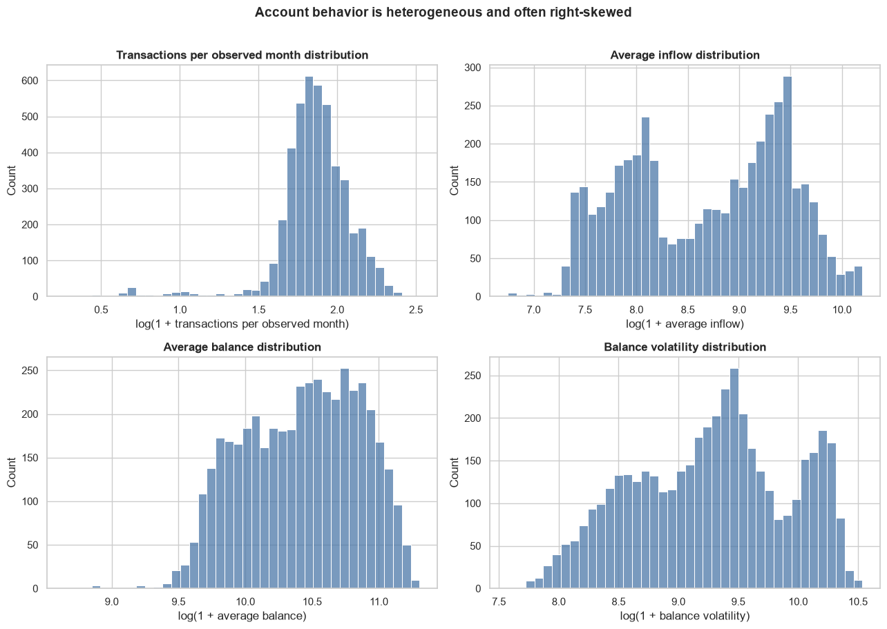
  • Are account balance profiles and service breadth heterogeneous?
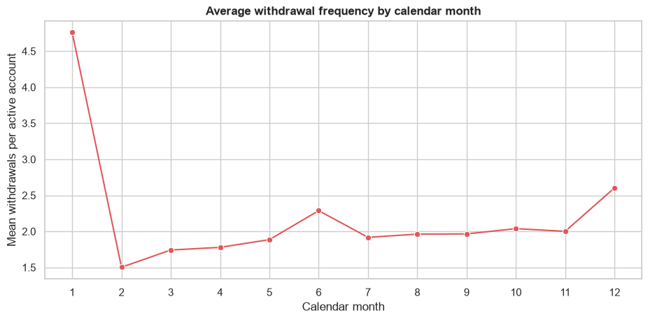
  • Do withdrawal patterns vary by calendar month?
  • Which observed service combinations occur more often than expected under independence?

2. Reproducible setup and Silver inputs

Notebook 1 created the validated Silver inputs used here. The local DuckDB database is accessed only for the standing-order purpose codes that are not present in the account Parquet table; ingestion and cleaning are not repeated.

Code
from pathlib import Path
import platform
import warnings

import duckdb
import matplotlib.pyplot as plt
import mlxtend
import numpy as np
import pandas as pd
import seaborn as sns
import statsmodels
from IPython.display import display
from mlxtend.frequent_patterns import apriori, association_rules
from sklearn.metrics import mean_absolute_error, root_mean_squared_error
from statsmodels.graphics.tsaplots import plot_acf, plot_pacf
from statsmodels.tools.sm_exceptions import ConvergenceWarning
from statsmodels.tsa.seasonal import seasonal_decompose
from statsmodels.tsa.stattools import adfuller
from statsmodels.tsa.statespace.sarimax import SARIMAX


def find_project_root(start: Path | None = None) -> Path:
    current = (start or Path.cwd()).resolve()
    for candidate in (current, *current.parents):
        if (candidate / "pyproject.toml").is_file():
            return candidate
    raise FileNotFoundError("Could not locate the project root containing pyproject.toml")


def sql_literal(path: Path) -> str:
    return "'" + str(path).replace("'", "''") + "'"


PROJECT_ROOT = find_project_root()
INTERIM_DIR = PROJECT_ROOT / "data" / "interim"
PROCESSED_DIR = PROJECT_ROOT / "data" / "processed"
DATABASE_PATH = INTERIM_DIR / "berka.duckdb"

TRANSACTIONS_PATH = INTERIM_DIR / "transactions_clean.parquet"
ACCOUNTS_CLIENTS_PATH = INTERIM_DIR / "accounts_clients.parquet"
LOANS_PATH = INTERIM_DIR / "loans_clean.parquet"
ACCOUNT_BASE_PATH = INTERIM_DIR / "account_analytical_base.parquet"

PROCESSED_DIR.mkdir(parents=True, exist_ok=True)

sns.set_theme(style="whitegrid", context="notebook")
plt.rcParams.update({"figure.figsize": (11, 5.5), "axes.titleweight": "bold"})

environment = pd.Series(
    {
        "Python": platform.python_version(),
        "DuckDB": duckdb.__version__,
        "pandas": pd.__version__,
        "statsmodels": statsmodels.__version__,
        "mlxtend": mlxtend.__version__,
        "Project root": ".",
    },
    name="value",
)
display(environment.to_frame())
value
Python 3.14.6
DuckDB 1.5.5
pandas 3.0.5
statsmodels 0.14.6
mlxtend 0.25.0
Project root .
Code
required_inputs = {
    "Local DuckDB database": DATABASE_PATH,
    "Clean transactions": TRANSACTIONS_PATH,
    "Account-client relationships": ACCOUNTS_CLIENTS_PATH,
    "Clean loans": LOANS_PATH,
    "Account analytical base": ACCOUNT_BASE_PATH,
}

input_status = pd.DataFrame(
    [
        {
            "input": name,
            "path": str(path.relative_to(PROJECT_ROOT)),
            "exists": path.is_file(),
            "size_mb": round(path.stat().st_size / 1_048_576, 3) if path.is_file() else None,
        }
        for name, path in required_inputs.items()
    ]
)
display(input_status)
assert input_status["exists"].all(), "Run Notebook 1 before this notebook."

connection = duckdb.connect(str(DATABASE_PATH), read_only=True)
transactions_scan = "read_parquet(" + sql_literal(TRANSACTIONS_PATH) + ")"
accounts_clients_scan = "read_parquet(" + sql_literal(ACCOUNTS_CLIENTS_PATH) + ")"
loans_scan = "read_parquet(" + sql_literal(LOANS_PATH) + ")"
account_base_scan = "read_parquet(" + sql_literal(ACCOUNT_BASE_PATH) + ")"

account_base = connection.execute("SELECT * FROM " + account_base_scan).fetchdf()
loans = connection.execute("SELECT * FROM " + loans_scan).fetchdf()

inventory = connection.execute(
    "SELECT 'transactions' AS dataset, COUNT(*) AS rows, COUNT(DISTINCT account_id) AS accounts FROM "
    + transactions_scan
    + " UNION ALL SELECT 'account base', COUNT(*), COUNT(DISTINCT account_id) FROM "
    + account_base_scan
    + " UNION ALL SELECT 'loans', COUNT(*), COUNT(DISTINCT account_id) FROM "
    + loans_scan
    + " UNION ALL SELECT 'account-client relationships', COUNT(*), COUNT(DISTINCT account_id) FROM "
    + accounts_clients_scan
).fetchdf()
display(inventory)

assert len(account_base) == account_base["account_id"].nunique() == 4_500
assert len(loans) == loans["loan_id"].nunique() == 682
input path exists size_mb
0 Local DuckDB database data/interim/berka.duckdb True 46.262
1 Clean transactions data/interim/transactions_clean.parquet True 7.636
2 Account-client relationships data/interim/accounts_clients.parquet True 0.065
3 Clean loans data/interim/loans_clean.parquet True 0.010
4 Account analytical base data/interim/account_analytical_base.parquet True 0.121
dataset rows accounts
0 transactions 1056320 4500
1 account base 4500 4500
2 loans 682 682
3 account-client relationships 5369 4500

3. Week 2 — Exploratory Data Analysis and Visualization

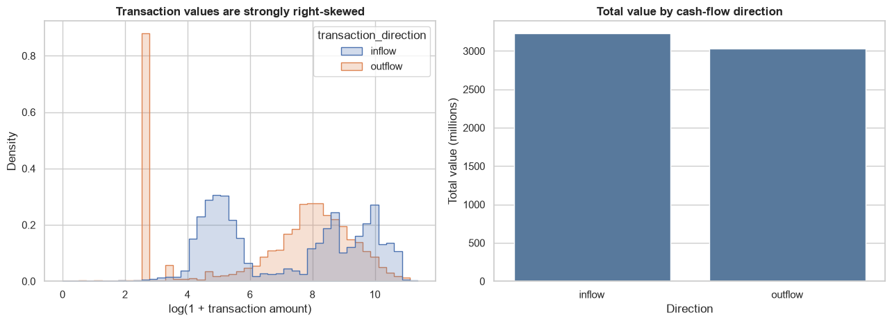
The exploration proceeds from the full portfolio to account-level behavior. Numerical summaries use all observations. A deterministic subset is used only for dense transaction-distribution plots so that visualization remains responsive and reproducible.

Code
transaction_summary = connection.execute(
    '''
    SELECT
        COUNT(*) AS transactions,
        COUNT(DISTINCT account_id) AS accounts,
        MIN(transaction_date) AS first_date,
        MAX(transaction_date) AS last_date,
        AVG(amount) AS mean_amount,
        MEDIAN(amount) AS median_amount,
        STDDEV_SAMP(amount) AS amount_std,
        QUANTILE_CONT(amount, 0.95) AS amount_p95,
        MAX(amount) AS maximum_amount,
        AVG(balance) AS transaction_weighted_mean_balance,
        MEDIAN(balance) AS transaction_weighted_median_balance,
        COUNT(*) FILTER (WHERE balance < 0) AS negative_balance_rows
    FROM '''
    + transactions_scan
).fetchdf()
display(transaction_summary.T.rename(columns={0: "value"}))

direction_profile = connection.execute(
    '''
    SELECT
        transaction_direction,
        COUNT(*) AS transaction_count,
        COUNT(DISTINCT account_id) AS account_count,
        SUM(amount) AS total_value,
        AVG(amount) AS mean_value,
        MEDIAN(amount) AS median_value
    FROM '''
    + transactions_scan
    + " GROUP BY 1 ORDER BY 1"
).fetchdf()
display(direction_profile)
value
transactions 1056320
accounts 4500
first_date 1993-01-01 00:00:00
last_date 1998-12-31 00:00:00
mean_amount 5924.210653
median_amount 2100.0
amount_std 9522.698104
amount_p95 25700.0
maximum_amount 87400
transaction_weighted_mean_balance 38518.379134
transaction_weighted_median_balance 33143.0
negative_balance_rows 2999
transaction_direction transaction_count account_count total_value mean_value median_value
0 inflow 405083 4500 3.227483e+09 7967.460160 1600.0
1 outflow 651237 4500 3.030380e+09 4653.266834 2128.0
Code
transaction_sample = connection.execute(
    '''
    SELECT transaction_direction, amount, balance
    FROM '''
    + transactions_scan
    + " WHERE trans_id % 10 = 0"
).fetchdf()

fig, axes = plt.subplots(1, 2, figsize=(13, 4.8))
sns.histplot(
    data=transaction_sample,
    x=np.log1p(transaction_sample["amount"]),
    hue="transaction_direction",
    element="step",
    stat="density",
    common_norm=False,
    bins=45,
    ax=axes[0],
)
axes[0].set(title="Transaction values are strongly right-skewed", xlabel="log(1 + transaction amount)")

direction_plot = direction_profile.assign(total_value_millions=lambda frame: frame["total_value"] / 1_000_000)
sns.barplot(data=direction_plot, x="transaction_direction", y="total_value_millions", ax=axes[1], color="#4C78A8")
axes[1].set(title="Total value by cash-flow direction", xlabel="Direction", ylabel="Total value (millions)")
fig.tight_layout()
plt.show()

Code
operation_profile = connection.execute(
    '''
    SELECT
        COALESCE(operation, 'not_recorded') AS operation,
        COUNT(*) AS transaction_count,
        COUNT(DISTINCT account_id) AS account_count,
        SUM(amount) AS total_value
    FROM '''
    + transactions_scan
    + " GROUP BY 1 ORDER BY transaction_count DESC"
).fetchdf()

purpose_profile = connection.execute(
    '''
    SELECT
        transaction_purpose,
        COUNT(*) AS transaction_count,
        COUNT(DISTINCT account_id) AS account_count,
        SUM(amount) AS total_value
    FROM '''
    + transactions_scan
    + " GROUP BY 1 ORDER BY transaction_count DESC"
).fetchdf()

display(operation_profile)
display(purpose_profile)

fig, axes = plt.subplots(1, 2, figsize=(14, 5.2))
sns.barplot(data=operation_profile, y="operation", x="transaction_count", ax=axes[0], color="#59A14F")
axes[0].set(title="Transaction operations", xlabel="Transactions", ylabel="")
sns.barplot(data=purpose_profile, y="transaction_purpose", x="transaction_count", ax=axes[1], color="#F28E2B")
axes[1].set(title="Recorded transaction purposes", xlabel="Transactions", ylabel="")
fig.tight_layout()
plt.show()
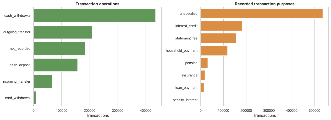
operation transaction_count account_count total_value
0 cash_withdrawal 434918 4500 2.339571e+09
1 outgoing_transfer 208283 3602 6.726385e+08
2 not_recorded 183114 4453 2.747976e+07
3 cash_deposit 156743 4500 2.418523e+09
4 incoming_transfer 65226 1606 7.814800e+08
5 card_withdrawal 8036 807 1.817040e+07
transaction_purpose transaction_count account_count total_value
0 unspecified 535314 4500 5.482194e+09
1 interest_credit 183114 4453 2.747976e+07
2 statement_fee 155832 4396 2.744045e+06
3 household_payment 118065 3297 4.985064e+08
4 pension 30338 740 1.674721e+08
5 insurance 18500 510 2.417519e+07
6 loan_payment 13580 682 5.525300e+07
7 penalty_interest 1577 264 3.773600e+04

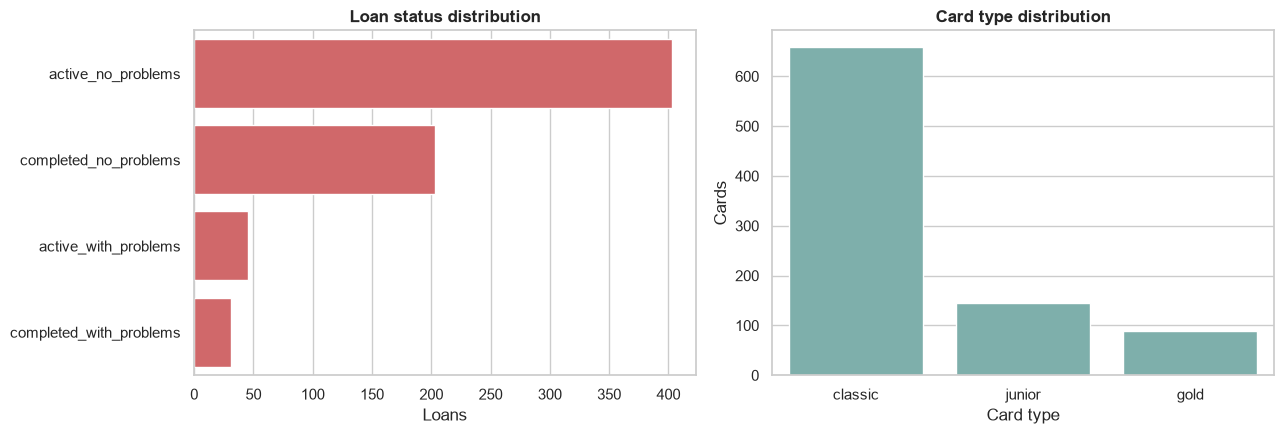
Loan, card, and district context

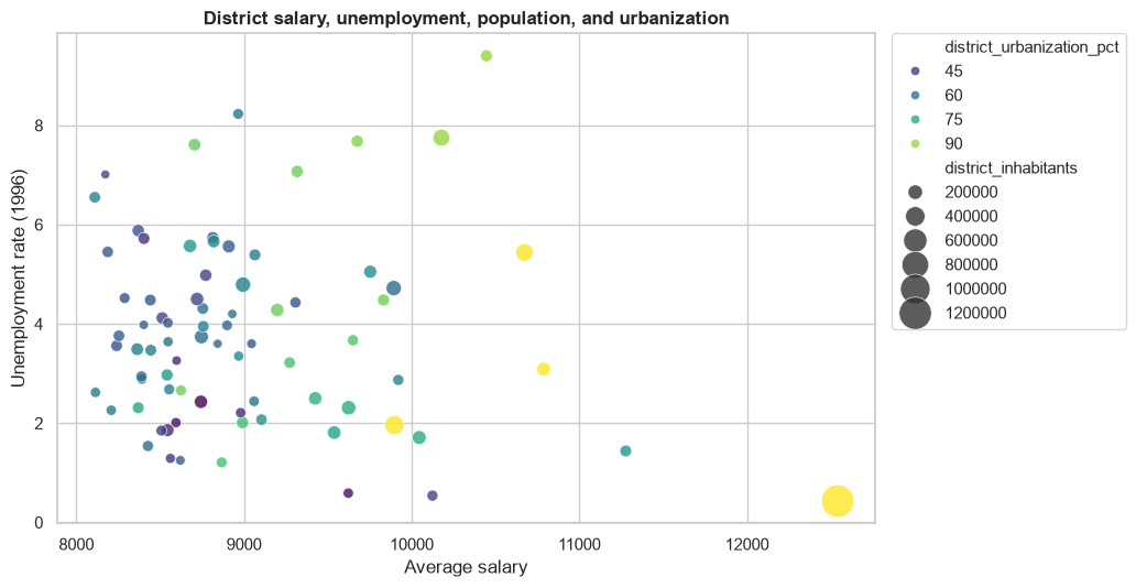
Loan and card characteristics describe service adoption, not customer quality. District statistics are analyzed at one row per district; using one row per account would unintentionally weight districts by this bank’s customer count.

Code
loan_profile = (
    loans.groupby("loan_status", dropna=False)
    .agg(loans=("loan_id", "size"), median_amount=("loan_amount", "median"), median_duration=("duration_months", "median"))
    .reset_index()
    .sort_values("loans", ascending=False)
)
card_profile = connection.execute(
    "SELECT type AS card_type, COUNT(*) AS cards FROM card GROUP BY 1 ORDER BY cards DESC"
).fetchdf()

display(loan_profile)
display(card_profile)

fig, axes = plt.subplots(1, 2, figsize=(13, 4.5))
sns.barplot(data=loan_profile, y="loan_status", x="loans", ax=axes[0], color="#E15759")
axes[0].set(title="Loan status distribution", xlabel="Loans", ylabel="")
sns.barplot(data=card_profile, x="card_type", y="cards", ax=axes[1], color="#76B7B2")
axes[1].set(title="Card type distribution", xlabel="Card type", ylabel="Cards")
fig.tight_layout()
plt.show()
loan_status loans median_amount median_duration
0 active_no_problems 403 153504.0 48.0
2 completed_no_problems 203 79632.0 24.0
1 active_with_problems 45 260400.0 48.0
3 completed_with_problems 31 96396.0 24.0
card_type cards
0 classic 659
1 junior 145
2 gold 88

Code
district_columns = [
    "account_district_id",
    "account_district_name",
    "district_inhabitants",
    "district_urbanization_pct",
    "district_average_salary",
    "district_unemployment_1995",
    "district_unemployment_1996",
    "district_entrepreneurs_per_1000",
    "district_crimes_1995",
    "district_crimes_1996",
]
districts = account_base[district_columns].drop_duplicates("account_district_id").reset_index(drop=True)
display(districts.drop(columns=["account_district_id", "account_district_name"]).describe().T)

district_plot = districts.dropna(subset=["district_average_salary", "district_unemployment_1996"])
fig, ax = plt.subplots(figsize=(10.5, 5.5))
sns.scatterplot(
    data=district_plot,
    x="district_average_salary",
    y="district_unemployment_1996",
    size="district_inhabitants",
    hue="district_urbanization_pct",
    sizes=(35, 450),
    palette="viridis",
    alpha=0.8,
    ax=ax,
)
ax.set(
    title="District salary, unemployment, population, and urbanization",
    xlabel="Average salary",
    ylabel="Unemployment rate (1996)",
)
ax.legend(bbox_to_anchor=(1.02, 1), loc="upper left", borderaxespad=0)
fig.tight_layout()
plt.show()
count mean std min 25% 50% 75% max
district_inhabitants 77.0 133884.896104 136913.464909 42821.0 85852.0 108871.0 139012.0 1204953.0
district_urbanization_pct 77.0 63.035065 16.221727 33.9 51.9 59.8 73.5 100.0
district_average_salary 77.0 9031.675325 790.202347 8110.0 8512.0 8814.0 9317.0 12541.0
district_unemployment_1995 76.0 3.072368 1.664179 0.2 1.7 2.8 3.85 7.3
district_unemployment_1996 77.0 3.787013 1.90848 0.43 2.31 3.6 4.79 9.4
district_entrepreneurs_per_1000 77.0 116.12987 16.608773 81.0 105.0 113.0 126.0 167.0
district_crimes_1995 76.0 4850.315789 9888.951933 818.0 2029.75 2932.0 4525.5 85677.0
district_crimes_1996 77.0 5030.831169 11270.796786 888.0 2122.0 3040.0 4595.0 99107.0

Temporal activity and resampling

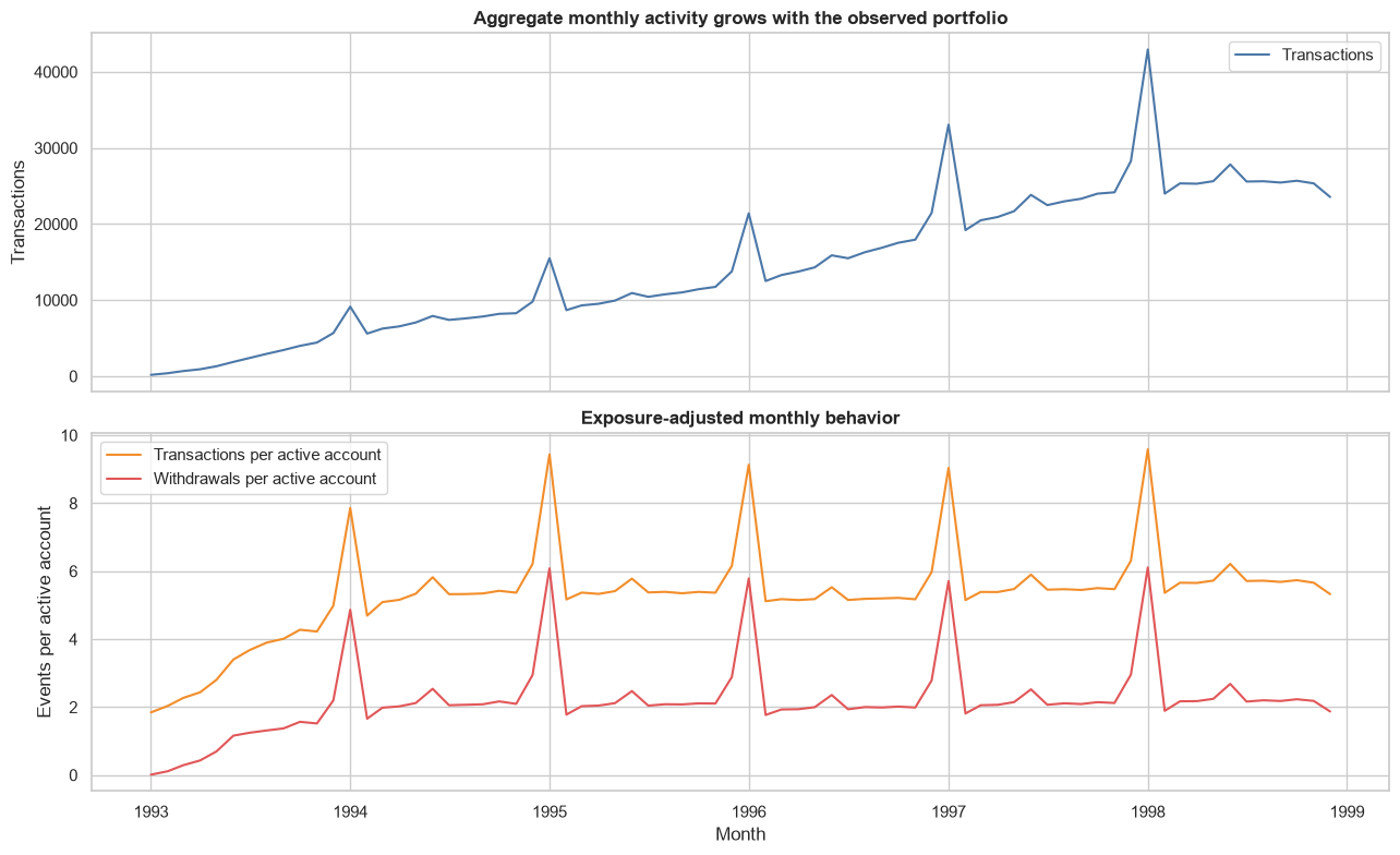
Transactions are irregular events. Daily counts and values are first aggregated in DuckDB and then resampled to regular month-start intervals with pandas. Monthly distinct active-account counts are calculated separately because daily distinct counts cannot be summed without double-counting accounts.

Code
daily_activity = connection.execute(
    '''
    SELECT
        transaction_date AS activity_date,
        COUNT(*) AS transaction_count,
        SUM(amount) FILTER (WHERE transaction_direction = 'inflow') AS total_inflow,
        SUM(amount) FILTER (WHERE transaction_direction = 'outflow') AS total_outflow,
        COUNT(*) FILTER (
            WHERE operation IN ('cash_withdrawal', 'card_withdrawal')
        ) AS withdrawal_count,
        SUM(amount) FILTER (
            WHERE operation IN ('cash_withdrawal', 'card_withdrawal')
        ) AS withdrawal_value
    FROM '''
    + transactions_scan
    + " GROUP BY 1 ORDER BY 1"
).fetchdf()

daily_activity["activity_date"] = pd.to_datetime(daily_activity["activity_date"])
monthly_activity = (
    daily_activity.set_index("activity_date")
    .resample("MS")
    .sum()
    .rename_axis("month")
    .reset_index()
)

monthly_accounts = connection.execute(
    '''
    SELECT
        DATE_TRUNC('month', transaction_date) AS month,
        COUNT(DISTINCT account_id) AS active_account_count
    FROM '''
    + transactions_scan
    + " GROUP BY 1 ORDER BY 1"
).fetchdf()
monthly_accounts["month"] = pd.to_datetime(monthly_accounts["month"])

monthly_activity = monthly_activity.merge(monthly_accounts, on="month", validate="one_to_one")
monthly_activity["net_cash_flow"] = monthly_activity["total_inflow"] - monthly_activity["total_outflow"]
monthly_activity["transactions_per_active_account"] = (
    monthly_activity["transaction_count"] / monthly_activity["active_account_count"]
)
monthly_activity["withdrawals_per_active_account"] = (
    monthly_activity["withdrawal_count"] / monthly_activity["active_account_count"]
)
monthly_activity["inflow_per_active_account"] = (
    monthly_activity["total_inflow"] / monthly_activity["active_account_count"]
)
monthly_activity["outflow_per_active_account"] = (
    monthly_activity["total_outflow"] / monthly_activity["active_account_count"]
)
monthly_activity["month_number"] = monthly_activity["month"].dt.month

expected_months = pd.date_range(monthly_activity["month"].min(), monthly_activity["month"].max(), freq="MS")
assert monthly_activity["month"].tolist() == expected_months.tolist()
assert len(monthly_activity) == 72
display(monthly_activity.head())
month transaction_count total_inflow total_outflow withdrawal_count withdrawal_value active_account_count net_cash_flow transactions_per_active_account withdrawals_per_active_account inflow_per_active_account outflow_per_active_account month_number
0 1993-01-01 177 667459.0 34700.0 1 34700.0 96 632759.0 1.843750 0.010417 6952.697917 361.458333 1
1 1993-02-01 395 2445507.0 281427.0 22 271815.0 194 2164080.0 2.036082 0.113402 12605.706186 1450.654639 2
2 1993-03-01 676 3855641.0 874690.0 86 852494.0 298 2980951.0 2.268456 0.288591 12938.392617 2935.201342 3
3 1993-04-01 913 5325769.0 2052623.0 161 2026940.0 375 3273146.0 2.434667 0.429333 14202.050667 5473.661333 4
4 1993-05-01 1306 7664745.0 4016046.0 324 3897139.0 466 3648699.0 2.802575 0.695279 16447.950644 8618.124464 5
Code
fig, axes = plt.subplots(2, 1, figsize=(13, 8), sharex=True)
axes[0].plot(monthly_activity["month"], monthly_activity["transaction_count"], label="Transactions", color="#4C78A8")
axes[0].set(title="Aggregate monthly activity grows with the observed portfolio", ylabel="Transactions")
axes[0].legend()

axes[1].plot(
    monthly_activity["month"],
    monthly_activity["transactions_per_active_account"],
    label="Transactions per active account",
    color="#F28E2B",
)
axes[1].plot(
    monthly_activity["month"],
    monthly_activity["withdrawals_per_active_account"],
    label="Withdrawals per active account",
    color="#E15759",
)
axes[1].set(title="Exposure-adjusted monthly behavior", xlabel="Month", ylabel="Events per active account")
axes[1].legend()
fig.tight_layout()
plt.show()

month_of_year_profile = (
    monthly_activity.groupby("month_number")
    .agg(
        mean_transactions_per_account=("transactions_per_active_account", "mean"),
        mean_withdrawals_per_account=("withdrawals_per_active_account", "mean"),
        mean_net_cash_flow=("net_cash_flow", "mean"),
    )
    .reset_index()
)
display(month_of_year_profile)

fig, ax = plt.subplots(figsize=(11, 4.8))
sns.lineplot(
    data=month_of_year_profile,
    x="month_number",
    y="mean_withdrawals_per_account",
    marker="o",
    color="#E15759",
    ax=ax,
)
ax.set(
    title="Average withdrawal frequency by calendar month",
    xlabel="Calendar month",
    ylabel="Mean withdrawals per active account",
    xticks=range(1, 13),
)
plt.show()

month_number mean_transactions_per_account mean_withdrawals_per_account mean_net_cash_flow
0 1 7.815282 4.759455 -1.530175e+07
1 2 4.586935 1.503019 1.120530e+07
2 3 4.824957 1.741863 5.325868e+06
3 4 4.851470 1.778805 4.444096e+06
4 5 4.987472 1.885816 2.836150e+06
5 6 5.439840 2.287833 -3.642036e+06
6 7 5.115416 1.917749 5.937728e+06
7 8 5.164515 1.962312 3.887138e+06
8 9 5.171804 1.965011 4.188178e+06
9 10 5.255783 2.038410 3.088171e+06
10 11 5.209620 2.000899 3.204042e+06
11 12 5.824685 2.604741 7.677638e+06

4. Customer behavioral feature construction

Features use information available through the dataset end date. Rates normalize unequal account tenure; raw counts are retained for interpretation. Demographic attributes and loan outcomes are intentionally excluded from this behavioral feature table so they cannot silently drive clustering in Notebook 3.

Key definitions

Feature group Definition
Transaction frequency Transactions per observed month and per active month
Funding and spending Mean/total inflow and outflow, their ratio, and channel shares
Balance behavior Mean, median, standard deviation, minimum, maximum, latest, range, negative-balance share
Tenure and activity Months from account opening to dataset end; active months divided by observed months
Transaction diversity Distinct operations, purposes, and operation-purpose patterns
Service diversity Count of observed card, loan, standing-order, recurring-income, pension, household, insurance, and leasing indicators

Salary-like deposit heuristic

Berka does not explicitly identify salary payments. receives_salary_like_deposit therefore means an unlabeled incoming transfer from the same counterparty observed in at least three months, with mean value at least 10,000 and coefficient of variation at most 0.25. It is an inferred recurring-income pattern, not a verified salary.

Code
FEATURES_SQL = '''
WITH parameters AS (
    SELECT MAX(transaction_date) AS analysis_end_date
    FROM {transactions}
),
transaction_features AS (
    SELECT
        account_id,
        COUNT(*) AS transaction_count,
        COUNT(DISTINCT transaction_month) AS active_months,
        SUM(amount) FILTER (WHERE transaction_direction = 'inflow') AS total_inflow,
        AVG(amount) FILTER (WHERE transaction_direction = 'inflow') AS average_inflow,
        SUM(amount) FILTER (WHERE transaction_direction = 'outflow') AS total_outflow,
        AVG(amount) FILTER (WHERE transaction_direction = 'outflow') AS average_outflow,
        AVG(balance) AS average_balance,
        MEDIAN(balance) AS median_balance,
        STDDEV_SAMP(balance) AS balance_std,
        MIN(balance) AS minimum_balance,
        MAX(balance) AS maximum_balance,
        AVG((balance < 0)::INTEGER) AS negative_balance_share,
        COUNT(DISTINCT operation) AS operation_diversity,
        COUNT(DISTINCT transaction_purpose) FILTER (
            WHERE transaction_purpose <> 'unspecified'
        ) AS purpose_diversity,
        COUNT(DISTINCT COALESCE(operation, 'not_recorded') || ':' || transaction_purpose) AS transaction_diversity,
        AVG((operation = 'cash_deposit')::INTEGER) AS cash_deposit_share,
        AVG((operation IN ('cash_withdrawal', 'card_withdrawal'))::INTEGER) AS cash_withdrawal_share,
        AVG((operation = 'incoming_transfer')::INTEGER) AS incoming_transfer_share,
        MAX((transaction_purpose = 'pension')::INTEGER) > 0 AS receives_pension,
        MAX((transaction_purpose = 'household_payment')::INTEGER) > 0 AS has_household_transaction,
        MAX((transaction_purpose = 'insurance')::INTEGER) > 0 AS has_insurance_transaction
    FROM {transactions}
    GROUP BY account_id
),
latest_balance AS (
    SELECT account_id, balance AS latest_balance
    FROM {transactions}
    QUALIFY ROW_NUMBER() OVER (
        PARTITION BY account_id ORDER BY transaction_date DESC, trans_id DESC
    ) = 1
),
recurring_income_sources AS (
    SELECT
        account_id,
        counterparty_bank,
        counterparty_account,
        COUNT(DISTINCT transaction_month) AS active_months,
        AVG(amount) AS mean_amount,
        STDDEV_POP(amount) / NULLIF(AVG(amount), 0) AS amount_cv
    FROM {transactions}
    WHERE transaction_direction = 'inflow'
      AND operation = 'incoming_transfer'
      AND transaction_purpose = 'unspecified'
      AND counterparty_account IS NOT NULL
    GROUP BY account_id, counterparty_bank, counterparty_account
),
salary_like_accounts AS (
    SELECT DISTINCT account_id
    FROM recurring_income_sources
    WHERE active_months >= 3
      AND mean_amount >= 10000
      AND amount_cv <= 0.25
),
order_features AS (
    SELECT
        account_id,
        MAX((TRIM(k_symbol) = 'SIPO')::INTEGER) > 0 AS has_household_order,
        MAX((TRIM(k_symbol) = 'POJISTNE')::INTEGER) > 0 AS has_insurance_order,
        MAX((TRIM(k_symbol) = 'LEASING')::INTEGER) > 0 AS makes_leasing_payments
    FROM "order"
    GROUP BY account_id
),
combined AS (
    SELECT
        base.account_id,
        DATE_DIFF('month', DATE_TRUNC('month', base.account_open_date), DATE_TRUNC('month', p.analysis_end_date)) + 1 AS observed_months,
        DATE_DIFF('day', base.account_open_date, p.analysis_end_date) / 30.4375 AS account_tenure_months,
        tf.* EXCLUDE (
            account_id,
            receives_pension,
            has_household_transaction,
            has_insurance_transaction
        ),
        lb.latest_balance,
        base.card_count,
        base.loan_count,
        base.standing_order_count,
        base.has_card,
        base.has_loan,
        base.has_standing_order,
        salary.account_id IS NOT NULL AS receives_salary_like_deposit,
        tf.receives_pension,
        tf.has_household_transaction OR COALESCE(of.has_household_order, FALSE) AS pays_household_expenses,
        tf.has_insurance_transaction OR COALESCE(of.has_insurance_order, FALSE) AS pays_insurance,
        COALESCE(of.makes_leasing_payments, FALSE) AS makes_leasing_payments
    FROM {account_base} AS base
    CROSS JOIN parameters AS p
    JOIN transaction_features AS tf USING (account_id)
    JOIN latest_balance AS lb USING (account_id)
    LEFT JOIN salary_like_accounts AS salary USING (account_id)
    LEFT JOIN order_features AS of USING (account_id)
)
SELECT
    account_id,
    observed_months,
    account_tenure_months,
    transaction_count,
    active_months,
    active_months::DOUBLE / observed_months AS active_month_ratio,
    transaction_count::DOUBLE / observed_months AS transactions_per_observed_month,
    transaction_count::DOUBLE / active_months AS transactions_per_active_month,
    total_inflow,
    average_inflow,
    total_outflow,
    average_outflow,
    total_inflow / NULLIF(total_outflow, 0) AS inflow_to_outflow_ratio,
    average_balance,
    median_balance,
    balance_std,
    minimum_balance,
    maximum_balance,
    latest_balance,
    maximum_balance - minimum_balance AS balance_range,
    negative_balance_share,
    operation_diversity,
    purpose_diversity,
    transaction_diversity,
    cash_deposit_share,
    cash_withdrawal_share,
    incoming_transfer_share,
    card_count,
    loan_count,
    standing_order_count,
    has_card,
    has_loan,
    has_standing_order,
    receives_salary_like_deposit,
    receives_pension,
    pays_household_expenses,
    pays_insurance,
    makes_leasing_payments,
    has_card::INTEGER
        + has_loan::INTEGER
        + has_standing_order::INTEGER
        + receives_salary_like_deposit::INTEGER
        + receives_pension::INTEGER
        + pays_household_expenses::INTEGER
        + pays_insurance::INTEGER
        + makes_leasing_payments::INTEGER AS service_diversity
FROM combined
ORDER BY account_id
'''.format(transactions=transactions_scan, account_base=account_base_scan)

customer_features = connection.execute(FEATURES_SQL).fetchdf()
display(customer_features.head())
account_id observed_months account_tenure_months transaction_count active_months active_month_ratio transactions_per_observed_month transactions_per_active_month total_inflow average_inflow ... standing_order_count has_card has_loan has_standing_order receives_salary_like_deposit receives_pension pays_household_expenses pays_insurance makes_leasing_payments service_diversity
0 1 46 45.273101 239 46 1.0 5.195652 5.195652 194322.0 1905.117647 ... 1 False False True False False True False False 2
1 2 71 70.110883 478 71 1.0 6.732394 6.732394 1597055.0 10506.940789 ... 2 False True True True False True False False 4
2 3 18 17.806982 117 18 1.0 6.500000 6.500000 173062.0 3762.217391 ... 3 False False True False False True True False 3
3 4 35 34.299795 186 35 1.0 5.314286 5.314286 192349.0 2959.215385 ... 2 False False True False True True False False 3
4 5 20 19.055441 84 20 1.0 4.200000 4.200000 97489.0 2785.400000 ... 1 False False True False True True False False 3

5 rows × 39 columns

Code
required_feature_columns = [
    "account_id",
    "transactions_per_observed_month",
    "average_inflow",
    "average_outflow",
    "inflow_to_outflow_ratio",
    "average_balance",
    "balance_std",
    "account_tenure_months",
    "active_month_ratio",
    "transaction_diversity",
    "service_diversity",
    "has_card",
    "has_loan",
    "has_standing_order",
]

feature_validation = pd.Series(
    {
        "rows": len(customer_features),
        "unique accounts": customer_features["account_id"].nunique(),
        "duplicate account IDs": customer_features["account_id"].duplicated().sum(),
        "missing required values": customer_features[required_feature_columns].isna().sum().sum(),
        "active-month ratio outside [0, 1]": (~customer_features["active_month_ratio"].between(0, 1)).sum(),
        "negative transaction frequencies": (customer_features["transactions_per_observed_month"] < 0).sum(),
    },
    name="value",
)
display(feature_validation.to_frame())

assert feature_validation["rows"] == feature_validation["unique accounts"] == 4_500
assert feature_validation["duplicate account IDs"] == 0
assert feature_validation["missing required values"] == 0
assert feature_validation["active-month ratio outside [0, 1]"] == 0
assert feature_validation["negative transaction frequencies"] == 0

behavior_summary_columns = [
    "transactions_per_observed_month",
    "average_inflow",
    "average_outflow",
    "inflow_to_outflow_ratio",
    "average_balance",
    "balance_std",
    "negative_balance_share",
    "transaction_diversity",
    "service_diversity",
]
display(customer_features[behavior_summary_columns].describe(percentiles=[0.05, 0.25, 0.5, 0.75, 0.95]).T)
value
rows 4500
unique accounts 4500
duplicate account IDs 0
missing required values 0
active-month ratio outside [0, 1] 0
negative transaction frequencies 0
count mean std min 5% 25% 50% 75% 95% max
transactions_per_observed_month 4500.0 5.556085 1.357805 0.310345 3.866667 4.772727 5.437060 6.282967 7.949169 11.466667
average_inflow 4500.0 7769.773444 5456.384171 851.385714 1721.061844 2952.035692 6599.089783 11688.899123 17615.053205 26885.953846
average_outflow 4500.0 4639.951985 3403.181162 498.735294 992.696180 1838.164096 3622.122500 6598.153603 11401.931190 19742.525000
inflow_to_outflow_ratio 4500.0 1.168193 0.644022 0.795939 1.017729 1.048451 1.089594 1.166473 1.436129 28.071429
average_balance 4500.0 36667.910906 15165.627811 5711.346154 16469.924821 23570.904108 34696.579426 47818.727179 64392.250290 81192.816993
balance_std 4500.0 12979.936540 7929.293890 1946.771770 3609.342332 6412.822830 11175.539654 17155.036902 28621.383107 37690.442560
negative_balance_share 4500.0 0.002885 0.019018 0.000000 0.000000 0.000000 0.000000 0.000000 0.007692 0.376900
transaction_diversity 4500.0 5.874444 1.197358 2.000000 4.000000 5.000000 6.000000 7.000000 8.000000 10.000000
service_diversity 4500.0 2.404000 1.149188 0.000000 0.000000 2.000000 3.000000 3.000000 4.000000 6.000000
Code
plot_features = [
    ("transactions_per_observed_month", "Transactions per observed month"),
    ("average_inflow", "Average inflow"),
    ("average_balance", "Average balance"),
    ("balance_std", "Balance volatility"),
]

fig, axes = plt.subplots(2, 2, figsize=(13, 9))
for ax, (column, label) in zip(axes.flat, plot_features):
    values = customer_features[column]
    if values.min() >= 0:
        sns.histplot(np.log1p(values), bins=40, ax=ax, color="#4C78A8")
        ax.set_xlabel("log(1 + " + label.lower() + ")")
    else:
        sns.histplot(values, bins=40, ax=ax, color="#4C78A8")
        ax.set_xlabel(label)
    ax.set_title(label + " distribution")
fig.suptitle("Account behavior is heterogeneous and often right-skewed", y=1.01, fontsize=14, weight="bold")
fig.tight_layout()
plt.show()

Code
correlation_features = [
    "transactions_per_observed_month",
    "average_inflow",
    "average_outflow",
    "inflow_to_outflow_ratio",
    "average_balance",
    "balance_std",
    "negative_balance_share",
    "cash_deposit_share",
    "cash_withdrawal_share",
    "incoming_transfer_share",
    "transaction_diversity",
    "service_diversity",
]
spearman_correlation = customer_features[correlation_features].corr(method="spearman")

fig, ax = plt.subplots(figsize=(11, 9))
sns.heatmap(
    spearman_correlation,
    cmap="vlag",
    center=0,
    vmin=-1,
    vmax=1,
    square=True,
    linewidths=0.4,
    ax=ax,
)
ax.set_title("Spearman correlations among account behaviors")
fig.tight_layout()
plt.show()

upper_triangle = spearman_correlation.where(
    np.triu(np.ones(spearman_correlation.shape, dtype=bool), k=1)
)
strongest_pairs = (
    upper_triangle.stack()
    .rename("spearman_rho")
    .reset_index()
    .rename(columns={"level_0": "feature_a", "level_1": "feature_b"})
    .assign(abs_rho=lambda frame: frame["spearman_rho"].abs())
    .sort_values("abs_rho", ascending=False)
    .head(12)
)
display(strongest_pairs)

feature_a feature_b spearman_rho abs_rho
14 average_inflow average_outflow 0.928279 0.928279
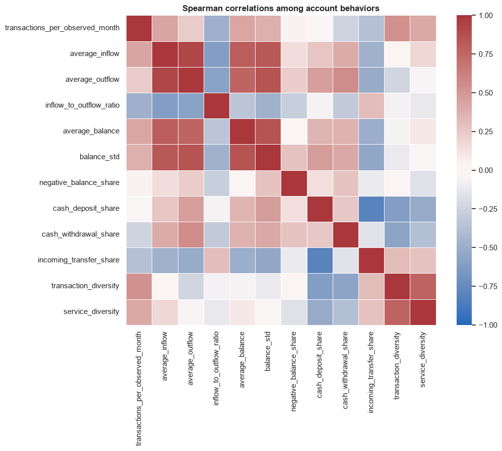
53 average_balance balance_std 0.858687 0.858687
29 average_outflow balance_std 0.858659 0.858659
17 average_inflow balance_std 0.831461 0.831461
16 average_inflow average_balance 0.807475 0.807475
93 cash_deposit_share incoming_transfer_share -0.807439 0.807439
131 transaction_diversity service_diversity 0.776768 0.776768
28 average_outflow average_balance 0.769096 0.769096
94 cash_deposit_share transaction_diversity -0.610223 0.610223
15 average_inflow inflow_to_outflow_ratio -0.609824 0.609824
27 average_outflow inflow_to_outflow_ratio -0.579228 0.579228
106 cash_withdrawal_share transaction_diversity -0.569978 0.569978
Code
funding_comparison = (
    customer_features.groupby("receives_salary_like_deposit")
    .agg(
        accounts=("account_id", "size"),
        median_average_inflow=("average_inflow", "median"),
        median_cash_deposit_share=("cash_deposit_share", "median"),
        median_incoming_transfer_share=("incoming_transfer_share", "median"),
        median_average_balance=("average_balance", "median"),
    )
    .reset_index()
)
display(funding_comparison)

behavioral_hypotheses = pd.DataFrame(
    [
        {
            "hypothesis": "Activity intensity may separate accounts.",
            "evidence to carry forward": "Wide account-level frequency distribution after tenure normalization.",
            "Notebook 3 implication": "Prefer rate features over raw lifetime transaction counts.",
        },
        {
            "hypothesis": "Funding channel may distinguish behavioral groups.",
            "evidence to carry forward": "Cash-deposit and incoming-transfer shares vary across accounts.",
            "Notebook 3 implication": "Compare channel shares and the salary-like indicator.",
        },
        {
            "hypothesis": "Liquidity level and volatility may form distinct profiles.",
            "evidence to carry forward": "Balance level, range, volatility, and negative-balance exposure differ.",
            "Notebook 3 implication": "Use robust transformations and avoid equating low balance with misconduct.",
        },
        {
            "hypothesis": "Service breadth may accompany behavioral complexity.",
            "evidence to carry forward": "Accounts vary in both transaction-pattern and service diversity.",
            "Notebook 3 implication": "Test whether service indicators improve interpretable clusters.",
        },
    ]
)
display(behavioral_hypotheses)
receives_salary_like_deposit accounts median_average_inflow median_cash_deposit_share median_incoming_transfer_share median_average_balance
0 False 4071 5694.364865 0.230769 0.000000 33693.442623
1 True 429 14542.740741 0.020173 0.197183 45743.129380
hypothesis evidence to carry forward Notebook 3 implication
0 Activity intensity may separate accounts. Wide account-level frequency distribution afte... Prefer rate features over raw lifetime transac...
1 Funding channel may distinguish behavioral gro... Cash-deposit and incoming-transfer shares vary... Compare channel shares and the salary-like ind...
2 Liquidity level and volatility may form distin... Balance level, range, volatility, and negative... Use robust transformations and avoid equating ...
3 Service breadth may accompany behavioral compl... Accounts vary in both transaction-pattern and ... Test whether service indicators improve interp...

5. Week 6 — Time Series Analysis and Forecasting

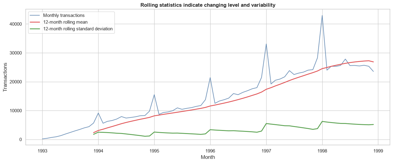
The primary series is monthly transaction count: an organizational workload measure with 72 equally spaced observations. Aggregate counts are affected by both customer behavior and the rapid expansion of observed accounts through 1997. Exposure-adjusted series are shown for diagnosis, but the forecast exercise remains at the requested organizational level.

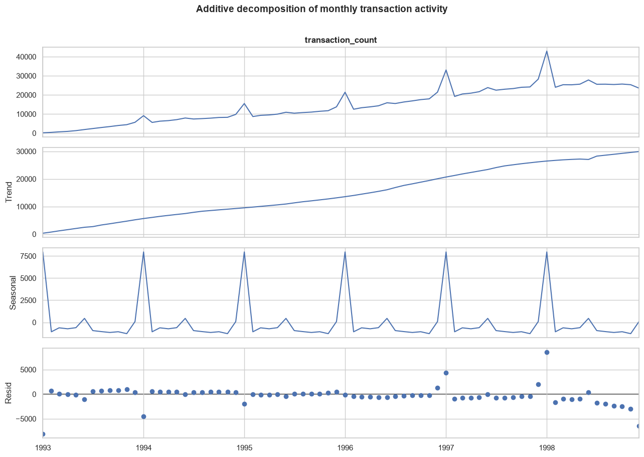
An additive seasonal period of 12 months is used. The final 12 months form an untouched chronological test set; no random split is appropriate for ordered observations.

Code
activity_series = monthly_activity.set_index("month")["transaction_count"].astype(float).asfreq("MS")
rolling_mean = activity_series.rolling(window=12).mean()
rolling_std = activity_series.rolling(window=12).std()

fig, ax = plt.subplots(figsize=(13, 5.5))
ax.plot(activity_series, label="Monthly transactions", color="#4C78A8", alpha=0.8)
ax.plot(rolling_mean, label="12-month rolling mean", color="#E15759", linewidth=2)
ax.plot(rolling_std, label="12-month rolling standard deviation", color="#59A14F", linewidth=2)
ax.set(title="Rolling statistics indicate changing level and variability", xlabel="Month", ylabel="Transactions")
ax.legend()
fig.tight_layout()
plt.show()

Code
decomposition = seasonal_decompose(activity_series, model="additive", period=12, extrapolate_trend="freq")
decomposition_figure = decomposition.plot()
decomposition_figure.set_size_inches(13, 9)
decomposition_figure.suptitle("Additive decomposition of monthly transaction activity", y=1.01, fontsize=14, weight="bold")
decomposition_figure.tight_layout()
plt.show()

Code
def adf_result(series: pd.Series, label: str) -> dict[str, float | str | int]:
    statistic, p_value, used_lags, observations, critical_values, _ = adfuller(series.dropna(), autolag="AIC")
    return {
        "series": label,
        "ADF statistic": statistic,
        "p_value": p_value,
        "used_lags": used_lags,
        "observations": observations,
        "critical_value_5pct": critical_values["5%"],
        "decision_at_0.05": "reject non-stationarity" if p_value <= 0.05 else "fail to reject non-stationarity",
    }


first_difference = activity_series.diff()
seasonal_first_difference = activity_series.diff(12).diff()
stationarity_results = pd.DataFrame(
    [
        adf_result(activity_series, "original monthly count"),
        adf_result(first_difference, "first difference"),
        adf_result(seasonal_first_difference, "seasonal + first difference"),
    ]
)
display(stationarity_results)

if (stationarity_results["p_value"] > 0.05).all():
    print(
        "The ADF test does not reject non-stationarity for any displayed transformation. "
        "Forecast results therefore require additional caution and holdout comparison."
    )
series ADF statistic p_value used_lags observations critical_value_5pct decision_at_0.05
0 original monthly count -1.307337 0.625809 12 59 -2.911939 fail to reject non-stationarity
1 first difference 0.110498 0.966771 11 59 -2.911939 fail to reject non-stationarity
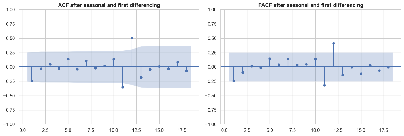
2 seasonal + first difference 0.841653 0.992280 11 47 -2.925338 fail to reject non-stationarity
The ADF test does not reject non-stationarity for any displayed transformation. Forecast results therefore require additional caution and holdout comparison.
Code
diagnostic_series = seasonal_first_difference.dropna()
fig, axes = plt.subplots(1, 2, figsize=(13, 4.5))
plot_acf(diagnostic_series, lags=18, zero=False, ax=axes[0])
plot_pacf(diagnostic_series, lags=18, zero=False, method="ywm", ax=axes[1])
axes[0].set_title("ACF after seasonal and first differencing")
axes[1].set_title("PACF after seasonal and first differencing")
fig.tight_layout()
plt.show()

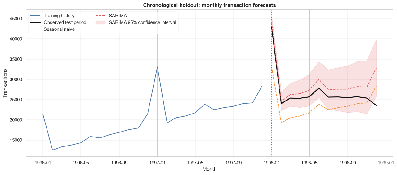
Chronological evaluation design

  • Training: first 60 months (1993-1997)
  • Test: final 12 months (1998)
  • Naive baselines: last observed value and the value from the same month one year earlier
  • Statistical model: SARIMA(1,1,1)(1,1,0,12), chosen as a compact demonstration consistent with trend and annual seasonality
  • Metrics: MAE and RMSE in transaction-count units

This is a single predeclared specification, not an exhaustive parameter search. With only 72 observations, extensive tuning would create unstable model-selection claims.

Code
TEST_MONTHS = 12
train = activity_series.iloc[:-TEST_MONTHS]
test = activity_series.iloc[-TEST_MONTHS:]

last_value_naive = pd.Series(train.iloc[-1], index=test.index, name="last_value_naive")
seasonal_naive = activity_series.shift(12).loc[test.index].rename("seasonal_naive")

with warnings.catch_warnings():
    warnings.simplefilter("ignore", ConvergenceWarning)
    warnings.simplefilter("ignore", DeprecationWarning)
    sarima_model = SARIMAX(
        train,
        order=(1, 1, 1),
        seasonal_order=(1, 1, 0, 12),
        trend="n",
        enforce_stationarity=False,
        enforce_invertibility=False,
    ).fit(disp=False)

sarima_result = sarima_model.get_forecast(steps=TEST_MONTHS)
sarima_forecast = sarima_result.predicted_mean.rename("sarima")
sarima_interval = sarima_result.conf_int(alpha=0.05)
residual_adf_p_value = adfuller(sarima_model.resid.iloc[14:], autolag="AIC")[1]

split_summary = pd.Series(
    {
        "training start": train.index.min().date(),
        "training end": train.index.max().date(),
        "test start": test.index.min().date(),
        "test end": test.index.max().date(),
        "training observations": len(train),
        "test observations": len(test),
        "SARIMA AIC": sarima_model.aic,
        "SARIMA BIC": sarima_model.bic,
        "SARIMA residual ADF p-value": residual_adf_p_value,
    },
    name="value",
)
display(split_summary.to_frame())
value
training start 1993-01-01
training end 1997-12-01
test start 1998-01-01
test end 1998-12-01
training observations 60
test observations 12
SARIMA AIC 556.671439
SARIMA BIC 562.776881
SARIMA residual ADF p-value 0.0
Code
forecast_candidates = {
    "Last-value naive": last_value_naive,
    "Seasonal naive": seasonal_naive,
    "SARIMA": sarima_forecast,
}
forecast_evaluation = pd.DataFrame(
    [
        {
            "model": name,
            "MAE": mean_absolute_error(test, prediction),
            "RMSE": root_mean_squared_error(test, prediction),
        }
        for name, prediction in forecast_candidates.items()
    ]
).sort_values("MAE").reset_index(drop=True)
display(forecast_evaluation)

forecast_index = train.index[-24:].append(test.index)
monthly_transaction_forecast = pd.DataFrame(
    {
        "month": forecast_index,
        "period": np.where(forecast_index < test.index.min(), "training", "test"),
        "observed_transaction_count": activity_series.reindex(forecast_index).astype("int64").to_numpy(),
        "seasonal_naive": seasonal_naive.reindex(forecast_index).to_numpy(),
        "sarima_forecast": sarima_forecast.reindex(forecast_index).to_numpy(),
        "sarima_lower_95": sarima_interval.iloc[:, 0].reindex(forecast_index).to_numpy(),
        "sarima_upper_95": sarima_interval.iloc[:, 1].reindex(forecast_index).to_numpy(),
    }
)
assert len(monthly_transaction_forecast) == 36
assert (monthly_transaction_forecast["period"] == "training").sum() == 24
assert (monthly_transaction_forecast["period"] == "test").sum() == 12
assert monthly_transaction_forecast.loc[
    monthly_transaction_forecast["period"] == "test",
    ["seasonal_naive", "sarima_forecast", "sarima_lower_95", "sarima_upper_95"],
].notna().all().all()

fig, ax = plt.subplots(figsize=(13, 5.8))
ax.plot(train.index[-24:], train.iloc[-24:], label="Training history", color="#4C78A8")
ax.plot(test, label="Observed test period", color="#111111", linewidth=2.2)
ax.plot(seasonal_naive, label="Seasonal naive", color="#F28E2B", linestyle="--")
ax.plot(sarima_forecast, label="SARIMA", color="#E15759", linestyle="--")
ax.fill_between(
    test.index,
    sarima_interval.iloc[:, 0].to_numpy(),
    sarima_interval.iloc[:, 1].to_numpy(),
    color="#E15759",
    alpha=0.18,
    label="SARIMA 95% confidence interval",
)
ax.axvline(test.index.min(), color="#777777", linestyle=":", linewidth=1.5)
ax.set(title="Chronological holdout: monthly transaction forecasts", xlabel="Month", ylabel="Transactions")
ax.legend(ncol=2)
fig.tight_layout()
plt.show()

best_forecast = forecast_evaluation.iloc[0]
print(
    f"Lowest holdout MAE: {best_forecast['model']} "
    f"({best_forecast['MAE']:,.0f} transactions; RMSE {best_forecast['RMSE']:,.0f})."
)
model MAE RMSE
0 SARIMA 2321.204834 3178.276490
1 Last-value naive 3857.750000 5145.290606
2 Seasonal naive 3941.666667 4494.930719

Lowest holdout MAE: SARIMA (2,321 transactions; RMSE 3,178).

Forecast interpretation limits

  • Confidence intervals describe parameter and residual uncertainty conditional on the fitted model; they do not cover every structural change.
  • Portfolio growth is a major driver of aggregate counts, so the series is not a pure measure of changing customer behavior.
  • January activity is visibly different from other months and may reflect recurring banking processes as well as customer behavior.
  • The 12-month holdout provides one evaluation window. It is adequate for a course demonstration but insufficient for production model selection.
  • Forecasting each account separately would create thousands of sparse, unstable models and is outside this project’s scope.

6. Week 7 — Recommendation Systems through Association Rules

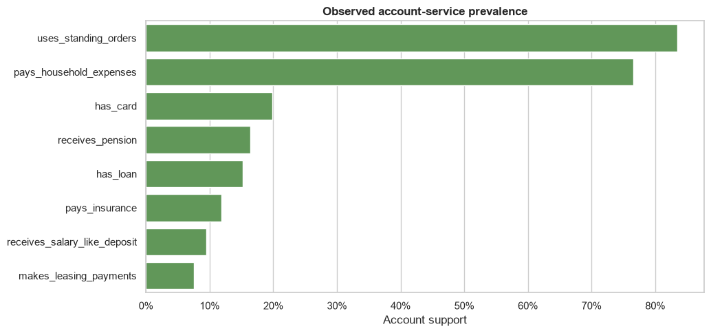
Berka contains no ratings, clicks, product catalogue, or response-to-recommendation outcomes. Collaborative filtering would therefore manufacture a preference signal that the dataset does not contain. A more defensible course connection is to treat each account as a basket of observed service and payment attributes.

The resulting rules answer: when attributes A and B are observed, how often is attribute C also observed, and is that co-occurrence greater than expected from C’s prevalence? They do not establish suitability, causation, customer interest, or incremental business value.

Code
service_columns = {
    "has_card": "has_card",
    "has_loan": "has_loan",
    "has_standing_order": "uses_standing_orders",
    "receives_salary_like_deposit": "receives_salary_like_deposit",
    "receives_pension": "receives_pension",
    "pays_household_expenses": "pays_household_expenses",
    "pays_insurance": "pays_insurance",
    "makes_leasing_payments": "makes_leasing_payments",
}
service_matrix = customer_features[list(service_columns)].rename(columns=service_columns).astype(bool)

service_prevalence = (
    service_matrix.mean()
    .sort_values(ascending=False)
    .rename("support")
    .to_frame()
    .assign(accounts=lambda frame: (frame["support"] * len(service_matrix)).round().astype(int))
)
display(service_prevalence)

fig, ax = plt.subplots(figsize=(10.5, 5))
sns.barplot(
    data=service_prevalence.reset_index().rename(columns={"index": "service"}),
    y="service",
    x="support",
    color="#59A14F",
    ax=ax,
)
ax.set(title="Observed account-service prevalence", xlabel="Account support", ylabel="")
ax.xaxis.set_major_formatter(plt.FuncFormatter(lambda value, _: f"{value:.0%}"))
fig.tight_layout()
plt.show()
support accounts
uses_standing_orders 0.835111 3758
pays_household_expenses 0.765111 3443
has_card 0.198222 892
receives_pension 0.164444 740
has_loan 0.151556 682
pays_insurance 0.118444 533
receives_salary_like_deposit 0.095333 429
makes_leasing_payments 0.075778 341

Code
MIN_SUPPORT = 0.03
MIN_CONFIDENCE = 0.35
MIN_LIFT = 1.05

frequent_itemsets = apriori(
    service_matrix,
    min_support=MIN_SUPPORT,
    use_colnames=True,
    max_len=3,
)
frequent_itemsets["item_count"] = frequent_itemsets["itemsets"].map(len)
frequent_itemsets = frequent_itemsets.sort_values(["item_count", "support"], ascending=[True, False])
display(frequent_itemsets.head(20))

all_rules = association_rules(
    frequent_itemsets,
    metric="confidence",
    min_threshold=MIN_CONFIDENCE,
)
all_rules["antecedent_count"] = all_rules["antecedents"].map(len)
all_rules["consequent_count"] = all_rules["consequents"].map(len)

standing_order_linked_services = {
    "has_loan",
    "pays_household_expenses",
    "pays_insurance",
    "makes_leasing_payments",
}


def is_structural_standing_order_rule(row: pd.Series) -> bool:
    rule_items = set(row["antecedents"]) | set(row["consequents"])
    return "uses_standing_orders" in rule_items and bool(rule_items & standing_order_linked_services)


candidate_rules = all_rules.loc[
    (all_rules["support"] >= MIN_SUPPORT)
    & (all_rules["confidence"] >= MIN_CONFIDENCE)
    & (all_rules["lift"] >= MIN_LIFT)
    & (all_rules["consequent_count"] == 1)
].copy()
candidate_rules["structural_standing_order_rule"] = candidate_rules.apply(
    is_structural_standing_order_rule,
    axis=1,
)
candidate_rules = candidate_rules.loc[~candidate_rules["structural_standing_order_rule"]].copy()
candidate_rules = candidate_rules.sort_values(["lift", "confidence", "support"], ascending=False)

display(
    candidate_rules[
        ["antecedents", "consequents", "support", "confidence", "lift", "leverage", "conviction"]
    ].head(15)
)
support itemsets item_count
2 0.835111 frozenset({uses_standing_orders}) 1
5 0.765111 frozenset({pays_household_expenses}) 1
0 0.198222 frozenset({has_card}) 1
4 0.164444 frozenset({receives_pension}) 1
1 0.151556 frozenset({has_loan}) 1
6 0.118444 frozenset({pays_insurance}) 1
3 0.095333 frozenset({receives_salary_like_deposit}) 1
7 0.075778 frozenset({makes_leasing_payments}) 1
17 0.754000 frozenset({pays_household_expenses, uses_stand... 2
21 0.164444 frozenset({receives_pension, pays_household_ex... 2
16 0.163556 frozenset({receives_pension, uses_standing_ord... 2
9 0.156000 frozenset({uses_standing_orders, has_card}) 2
12 0.151556 frozenset({uses_standing_orders, has_loan}) 2
11 0.132222 frozenset({pays_household_expenses, has_card}) 2
22 0.118444 frozenset({pays_household_expenses, pays_insur... 2
18 0.118222 frozenset({uses_standing_orders, pays_insurance}) 2
14 0.104000 frozenset({pays_household_expenses, has_loan}) 2
15 0.079778 frozenset({receives_salary_like_deposit, uses_... 2
19 0.075778 frozenset({makes_leasing_payments, uses_standi... 2
20 0.056222 frozenset({pays_household_expenses, receives_s... 2
antecedents consequents support confidence lift leverage conviction
37 frozenset({pays_household_expenses, receives_s... frozenset({has_loan}) 0.030667 0.545455 3.599040 0.022146 1.866578
13 frozenset({receives_salary_like_deposit}) frozenset({has_loan}) 0.046667 0.489510 3.229908 0.032218 1.662021
2 frozenset({receives_pension}) frozenset({pays_household_expenses}) 0.164444 1.000000 1.307000 0.038626 inf
7 frozenset({pays_insurance}) frozenset({pays_household_expenses}) 0.118444 1.000000 1.307000 0.027821 inf
3 frozenset({receives_pension}) frozenset({uses_standing_orders}) 0.163556 0.994595 1.190973 0.026226 30.504444
Code
association_rules_output = candidate_rules.copy()
association_rules_output["antecedents"] = association_rules_output["antecedents"].map(
    lambda items: " | ".join(sorted(items))
)
association_rules_output["consequents"] = association_rules_output["consequents"].map(
    lambda items: " | ".join(sorted(items))
)
association_rules_output["rule"] = (
    association_rules_output["antecedents"] + " -> " + association_rules_output["consequents"]
)
association_rules_output = association_rules_output.rename(
    columns={
        "antecedent support": "antecedent_support",
        "consequent support": "consequent_support",
    }
)
rule_output_columns = [
    "rule",
    "antecedents",
    "consequents",
    "antecedent_count",
    "consequent_count",
    "antecedent_support",
    "consequent_support",
    "support",
    "confidence",
    "lift",
    "leverage",
    "conviction",
]
association_rules_output = association_rules_output[rule_output_columns].reset_index(drop=True)

assert not association_rules_output.empty, "No recommendation hypotheses met the declared thresholds."
assert (association_rules_output["support"] >= MIN_SUPPORT).all()
assert (association_rules_output["confidence"] >= MIN_CONFIDENCE).all()
assert (association_rules_output["lift"] >= MIN_LIFT).all()

display(association_rules_output.head(15))

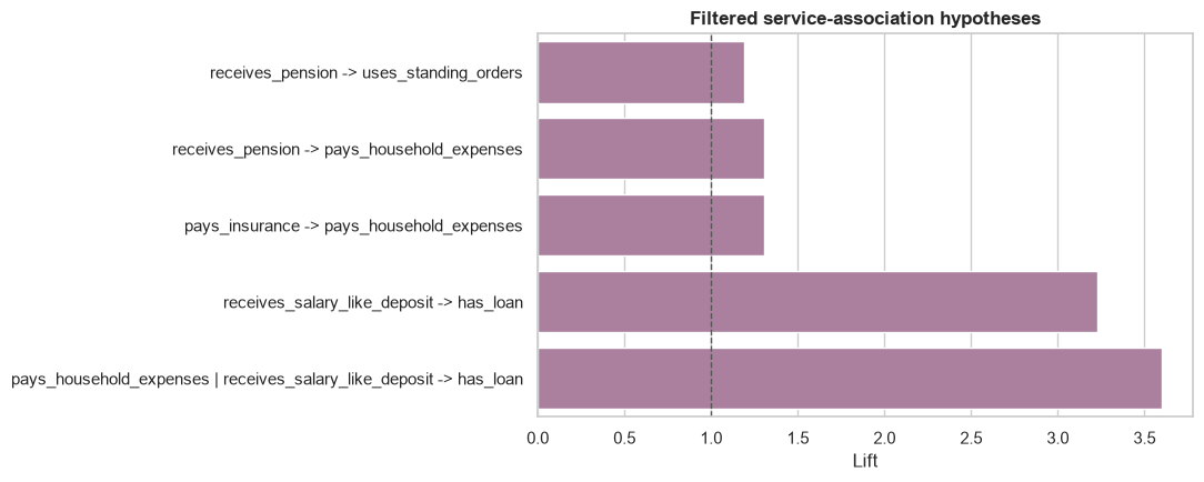
top_rules = association_rules_output.head(12).sort_values("lift")
fig, ax = plt.subplots(figsize=(11, max(4.5, 0.45 * len(top_rules))))
sns.barplot(data=top_rules, y="rule", x="lift", color="#B279A2", ax=ax)
ax.axvline(1, color="#555555", linestyle="--", linewidth=1)
ax.set(title="Filtered service-association hypotheses", xlabel="Lift", ylabel="")
fig.tight_layout()
plt.show()
rule antecedents consequents antecedent_count consequent_count antecedent_support consequent_support support confidence lift leverage conviction
0 pays_household_expenses | receives_salary_like... pays_household_expenses | receives_salary_like... has_loan 2 1 0.056222 0.151556 0.030667 0.545455 3.599040 0.022146 1.866578
1 receives_salary_like_deposit -> has_loan receives_salary_like_deposit has_loan 1 1 0.095333 0.151556 0.046667 0.489510 3.229908 0.032218 1.662021
2 receives_pension -> pays_household_expenses receives_pension pays_household_expenses 1 1 0.164444 0.765111 0.164444 1.000000 1.307000 0.038626 inf
3 pays_insurance -> pays_household_expenses pays_insurance pays_household_expenses 1 1 0.118444 0.765111 0.118444 1.000000 1.307000 0.027821 inf
4 receives_pension -> uses_standing_orders receives_pension uses_standing_orders 1 1 0.164444 0.835111 0.163556 0.994595 1.190973 0.026226 30.504444

How to read the rules

  • Support: proportion of all accounts containing the complete itemset.
  • Confidence: among accounts with the antecedent, proportion also containing the consequent.
  • Lift: observed co-occurrence divided by expected co-occurrence under independence; values above 1 indicate positive association.
  • Filtering: retained rules have support at least 3%, confidence at least 35%, lift at least 1.05, and one consequent.
  • Structural safeguards: rules connecting standing orders to services defined from standing-order records or loan repayment setup are removed because they partly restate the data construction.
  • Credit safeguard: loan-related associations are descriptive context only. They must not be used to approve, market, or recommend credit without suitability, fairness, and outcome evidence that Berka does not provide.

A surviving rule is a candidate for further investigation—for example, a future controlled study of service relevance—not permission to target an individual account.

7. Persist and validate Gold outputs

Output Grain Downstream purpose
customer_behavior_features.parquet One row per account Notebook 3 segmentation and profiling
monthly_banking_activity.parquet One row per calendar month Temporal reporting and forecast reproduction
monthly_transaction_forecast.parquet One row per displayed forecast month Dashboard holdout and uncertainty visualization
service_association_rules.parquet One row per filtered directional rule Recommendation-hypothesis review
Code
outputs = {
    "customer_behavior_features.parquet": customer_features,
    "monthly_banking_activity.parquet": monthly_activity,
    "monthly_transaction_forecast.parquet": monthly_transaction_forecast,
    "service_association_rules.parquet": association_rules_output,
}

for index, (filename, frame) in enumerate(outputs.items()):
    relation_name = f"notebook_output_{index}"
    output_path = PROCESSED_DIR / filename
    connection.register(relation_name, frame)
    connection.execute(
        "COPY (SELECT * FROM "
        + relation_name
        + ") TO "
        + sql_literal(output_path)
        + " (FORMAT PARQUET, COMPRESSION ZSTD)"
    )
    connection.unregister(relation_name)

output_validation_rows = []
for filename, frame in outputs.items():
    output_path = PROCESSED_DIR / filename
    stored_rows = connection.execute(
        "SELECT COUNT(*) FROM read_parquet(" + sql_literal(output_path) + ")"
    ).fetchone()[0]
    output_validation_rows.append(
        {
            "output": filename,
            "path": str(output_path.relative_to(PROJECT_ROOT)),
            "expected_rows": len(frame),
            "stored_rows": stored_rows,
            "columns": len(frame.columns),
            "size_kb": round(output_path.stat().st_size / 1024, 1),
            "valid": stored_rows == len(frame),
        }
    )

output_validation = pd.DataFrame(output_validation_rows)
display(output_validation)
assert output_validation["valid"].all()
output path expected_rows stored_rows columns size_kb valid
0 customer_behavior_features.parquet data/processed/customer_behavior_features.parquet 4500 4500 39 377.4 True
1 monthly_banking_activity.parquet data/processed/monthly_banking_activity.parquet 72 72 13 6.6 True
2 monthly_transaction_forecast.parquet data/processed/monthly_transaction_forecast.pa... 36 36 7 1.9 True
3 service_association_rules.parquet data/processed/service_association_rules.parquet 5 5 12 2.6 True

8. Findings and handoff

  • The observed portfolio grows from 96 active accounts in January 1993 to roughly 4,480 in most of 1998, so totals must be interpreted alongside exposure-adjusted behavior.
  • January has the highest average withdrawal frequency (4.76 withdrawals per active account); December is a distant second (2.60). This supports an annual-pattern hypothesis without identifying its cause.
  • Transaction value, activity intensity, funding channel, balance behavior, and service breadth provide distinct candidate dimensions for segmentation. Exactly 429 accounts meet the documented salary-like heuristic, which remains unverified.
  • Valid negative balances and extreme transaction values remain behavioral observations, not evidence of error or fraud.
  • Monthly transaction activity contains trend and annual seasonality. The ADF tests do not reject non-stationarity for the displayed transformations, although the fitted SARIMA residuals do; the short history and changing portfolio still limit forecast certainty.
  • SARIMA has the lowest 1998 holdout error in this declared comparison (MAE 2,321 transactions versus 3,858 for last-value naive and 3,942 for seasonal naive).
  • Service rules identify positive co-occurrence patterns only. They are recommendation hypotheses, not personalized recommendations or proof of unmet need.
  • Demographics and loan outcomes remain outside the clustering feature set and can be used later only for responsible post-hoc validation.

Next notebook: 03_customer_segmentation.ipynb will select and transform defensible behavioral features, compare clustering solutions, evaluate stability and separation, profile the resulting segments, and analyze contextual outliers without fraud labels.