This notebook is the analytical centre of the project. It selects defensible behavioral features, treats skewness and scale, interprets principal components, compares K-means with a Gaussian Mixture Model (GMM), evaluates stability and preprocessing sensitivity, profiles the selected segments, and investigates behavioral outliers.
It does not use demographics, loan outcomes, fraud labels, or t-SNE coordinates to construct the segments.
Notebook objectives
Select non-redundant behavioral features and document exclusions.
Apply skewness treatment and scaling through a reproducible pipeline.
Use PCA to interpret the major behavioral dimensions.
Compare K-means and GMM solutions across reasonable cluster counts.
Select a stable, interpretable segmentation using multiple criteria.
Describe every segment in behavioral and service terms.
Identify unusual accounts using four complementary, non-fraud outlier signals.
Persist three analytical tables and three fitted model artifacts.
1. Analytical contract
The unit of analysis is one bank account. Clusters summarize similarities in the historical Berka snapshot; they are not natural customer “types,” causal explanations, or eligibility categories.
Decision
Choice
Reason
Primary clustering family
K-means
Transparent centroid-based baseline and direct distance interpretation
Challenger
Gaussian Mixture Model
Probabilistic membership and flexible component covariance
Fuzzy C-means
Not implemented
GMM already demonstrates soft membership; adding FCM would expand scope without changing the central comparison
PCA
Interpretation and visualization
Linear components expose variance and loadings; full transformed features retain all information for primary clustering
t-SNE
Visualization only
Local neighborhoods may be useful visually, but global distances and apparent group sizes are distorted
Protected/context variables
Excluded from clustering
Gender, age, district, and loan outcomes must not silently define behavioral segments
Because this is descriptive unsupervised analysis, the preprocessing pipeline is fitted on the complete historical snapshot. Any future scoring workflow must reuse these fitted transformations and treat distribution shift as a new validation problem.
2. Reproducible setup and use of the Gold layer in the project’s medallion data architecture:
Notebook 2 produced one behavioral record per account. This notebook consumes that table without repeating transaction aggregation.
assert FEATURES_PATH.is_file(), "Run Notebook 2 before this notebook."connection = duckdb.connect()customer_features = connection.execute("SELECT * FROM read_parquet("+ sql_literal(FEATURES_PATH) +") ORDER BY account_id").fetchdf()input_validation = pd.Series( {"path": str(FEATURES_PATH.relative_to(PROJECT_ROOT)),"rows": len(customer_features),"columns": len(customer_features.columns),"unique accounts": customer_features["account_id"].nunique(),"duplicate account IDs": customer_features["account_id"].duplicated().sum(),"total missing values": customer_features.isna().sum().sum(), }, name="value",)display(input_validation.to_frame())assertlen(customer_features) == customer_features["account_id"].nunique() ==4_500assert customer_features["account_id"].duplicated().sum() ==0assert customer_features.isna().sum().sum() ==0
value
path
data/processed/customer_behavior_features.parquet
rows
4500
columns
39
unique accounts
4500
duplicate account IDs
0
total missing values
0
3. Pre-modelling analysis
Feature selection
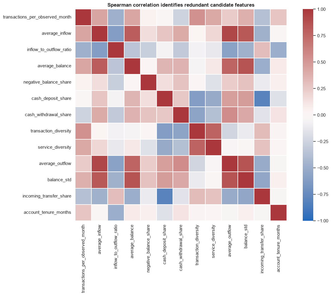
The selected representation balances four behavioral ideas: transaction intensity, cash-flow scale and coverage, balance condition, channel mix, and behavioral/service breadth. Lifetime totals and raw counts are excluded because unequal account tenure would dominate them. Highly redundant features remain available for profiling and sensitivity analysis.
Code
MODEL_FEATURES = ["transactions_per_observed_month","average_inflow","inflow_to_outflow_ratio","average_balance","negative_balance_share","cash_deposit_share","cash_withdrawal_share","transaction_diversity","service_diversity",]BEHAVIOR_ONLY_FEATURES = [ feature for feature in MODEL_FEATURES if feature !="service_diversity"]EXPANDED_FEATURES = MODEL_FEATURES + ["average_outflow","balance_std","incoming_transfer_share","account_tenure_months",]PROFILE_CONTINUOUS_FEATURES = ["transactions_per_observed_month","average_inflow","average_outflow","inflow_to_outflow_ratio","average_balance","balance_std","negative_balance_share","cash_deposit_share","cash_withdrawal_share","incoming_transfer_share","transaction_diversity","service_diversity",]SERVICE_INDICATORS = ["has_card","has_loan","has_standing_order","receives_salary_like_deposit","receives_pension","pays_household_expenses","pays_insurance","makes_leasing_payments",]feature_decisions = pd.DataFrame( [ {"feature or group": "transactions_per_observed_month","decision": "include","reason": "Average monthly transaction activity, adjusted for the account’s observation period.", }, {"feature or group": "average_inflow","decision": "include","reason": "Cash-flow scale; average outflow is reserved for profiling because the two are strongly correlated.", }, {"feature or group": "inflow_to_outflow_ratio","decision": "include","reason": "Relative funding coverage rather than another absolute value.", }, {"feature or group": "average_balance","decision": "include","reason": "Typical account balance level; balance variability is excluded from clustering to reduce redundancy and used afterward to describe the segments.", }, {"feature or group": "negative_balance_share","decision": "include","reason": "Frequency of a valid financial state, not a fraud or risk label.", }, {"feature or group": "cash_deposit_share, cash_withdrawal_share","decision": "include","reason": "Relative use of cash deposits and cash withdrawals among the account's transactions.", }, {"feature or group": "transaction_diversity, service_diversity","decision": "include","reason": "Summarizes transaction and service variety without allowing numerous rare service indicators to disproportionately influence clustering distances.", }, {"feature or group": "lifetime counts and totals","decision": "exclude","reason": "accounts were observed for different lengths of time. Older accounts naturally accumulate more transactions and larger totals, even if their monthly behavior is similar.", }, {"feature or group": "individual service flags","decision": "profile only","reason": "Used after clustering to describe each segment, without letting uncommon service indicators have too much influence on cluster formation", }, {"feature or group": "tenure, demographics, loan outcomes","decision": "context only","reason": "Avoid lifecycle, protected-attribute, and outcome-driven clusters.", }, ])display(feature_decisions)
feature or group
decision
reason
0
transactions_per_observed_month
include
Average monthly transaction activity, adjusted...
1
average_inflow
include
Cash-flow scale; average outflow is reserved f...
2
inflow_to_outflow_ratio
include
Relative funding coverage rather than another ...
3
average_balance
include
Typical account balance level; balance variabi...
4
negative_balance_share
include
Frequency of a valid financial state, not a fr...
5
cash_deposit_share, cash_withdrawal_share
include
Relative use of cash deposits and cash withdra...
6
transaction_diversity, service_diversity
include
Summarizes transaction and service variety wit...
7
lifetime counts and totals
exclude
accounts were observed for different lengths o...
8
individual service flags
profile only
Used after clustering to describe each segment...
9
tenure, demographics, loan outcomes
context only
Avoid lifecycle, protected-attribute, and outc...
Skewness treatment and scaling
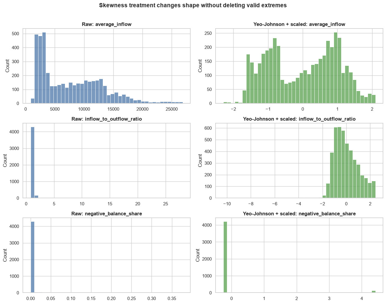
K-means is distance-based, and GMM is distribution-based. Both are sensitive to scale and extreme skew. The primary pipeline applies a fitted Yeo-Johnson transformation followed by standardization:
Yeo-Johnson: reduces skewness while supporting zeros. This is an additional preprocessing technique, used to reduce feature skewness while supporting zero-valued observations.
StandardScaler: gives every transformed feature mean approximately zero and variance one.
All accounts and valid extreme values are retained. Later, clustering with and without the Yeo-Johnson transformation is compared to determine how much this preprocessing choice affects the results.
Spearman correlation is used because many behaviors are non-normal and monotonic rather than linear. Correlation is a redundancy diagnostic here, not evidence of causation.
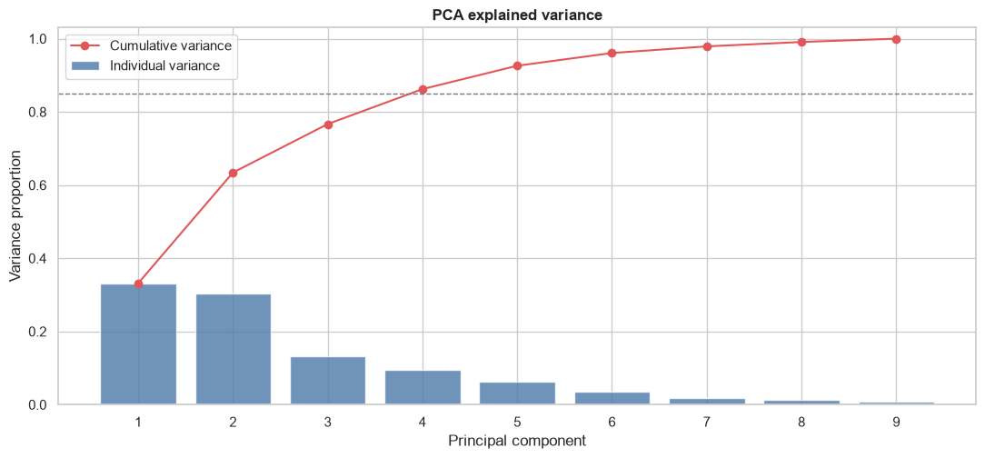
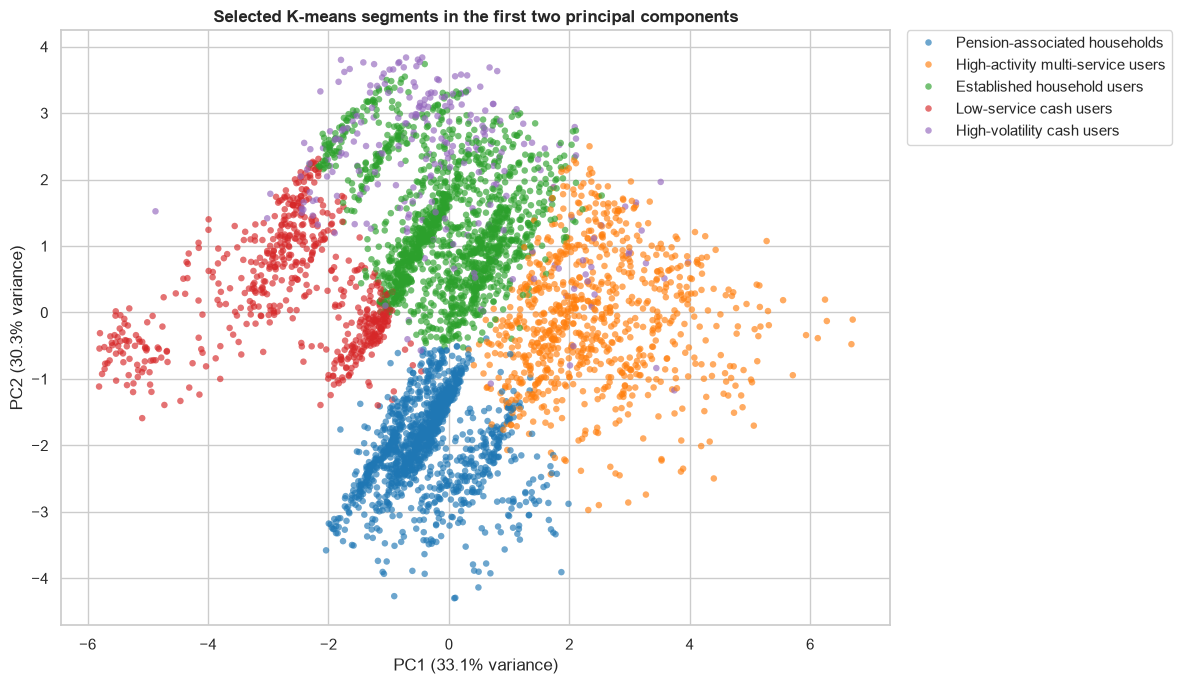
PCA is fitted to the transformed nine-feature matrix. It is used to quantify variance, interpret combinations of behavior through loadings, and visualize the selected segments. The primary clustering model remains in the full transformed feature space.
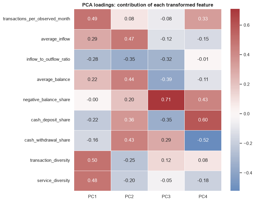
The first two components explain about 63% of transformed variance. PC1 primarily represents engagement breadth and activity intensity; PC2 emphasizes cash-flow and balance scale. Four components exceed 85%, so a four-component clustering sensitivity check is included later. Loading signs are arbitrary; relative magnitude and co-direction are what matter.
5. K-means baseline and value of K
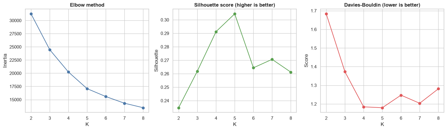
Candidate values from 2 through 8 are compared. Inertia supports the elbow method; silhouette rewards cohesion and separation; Davies-Bouldin rewards low within-to-between-cluster similarity. No single metric is treated as sufficient.
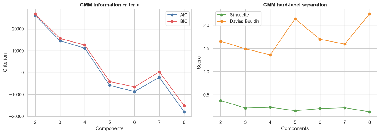
GMM provides soft membership probabilities and allows elliptical components through full covariance matrices. AIC and BIC are reported alongside hard-label silhouette and Davies-Bouldin scores. Lower AIC/BIC is preferable, but component likelihood alone does not guarantee useful customer segments.
The lowest tested GMM BIC occurs at K=8, the search boundary rather than a compact interior optimum.
K-means is retained as the primary model. At matched K=5 it provides materially better silhouette and Davies-Bouldin separation, produces operationally readable centroids, and supports direct centroid-distance outlier analysis. The GMM search reaches its lowest BIC at the upper boundary rather than a compact interior optimum, and the zero-inflated/discrete behaviors also strain a Gaussian assumption. GMM remains valuable as a challenger and as a source of membership uncertainty.
7. Stability and sensitivity
Adjusted Rand Index (ARI) compares assignments without depending on numeric cluster labels. ARI near 1 means two solutions assign nearly all account pairs consistently.
The sensitivity analysis supports three conclusions:
removing skewness treatment creates a nearly empty cluster, showing that untransformed extremes can dominate K-means;
removing service diversity or adding redundant/context variables changes some assignments but preserves substantial structure;
clustering the first four PCs produces nearly the same solution, supporting the selected structure while the full feature space retains the remaining variance.
Sensitivity is evidence about robustness, not proof that five “true” groups exist.
8. Selected segment visualization
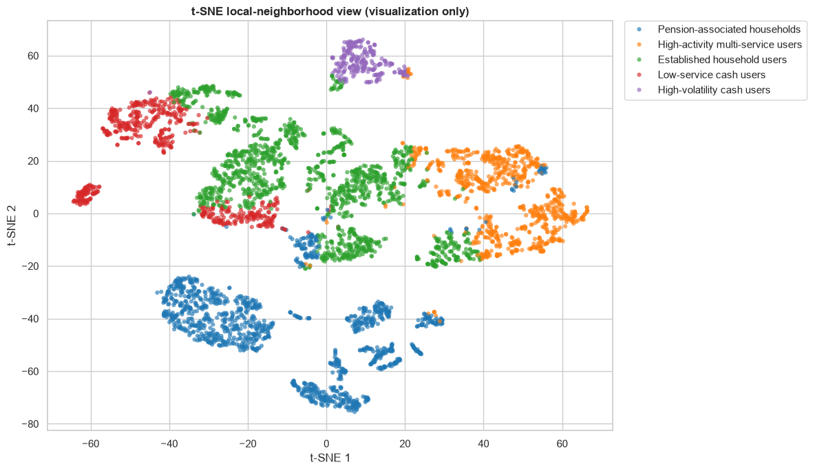
The numeric K-means labels are arbitrary. Stable descriptive names are attached only after reviewing original-scale profiles.
t-SNE is fitted only to create a second visual perspective on local neighborhoods. It is not used for K selection, clustering, stability, segment sizes, or outlier scores. Distances between separated groups and the visual area occupied by each color are not quantitatively meaningful.
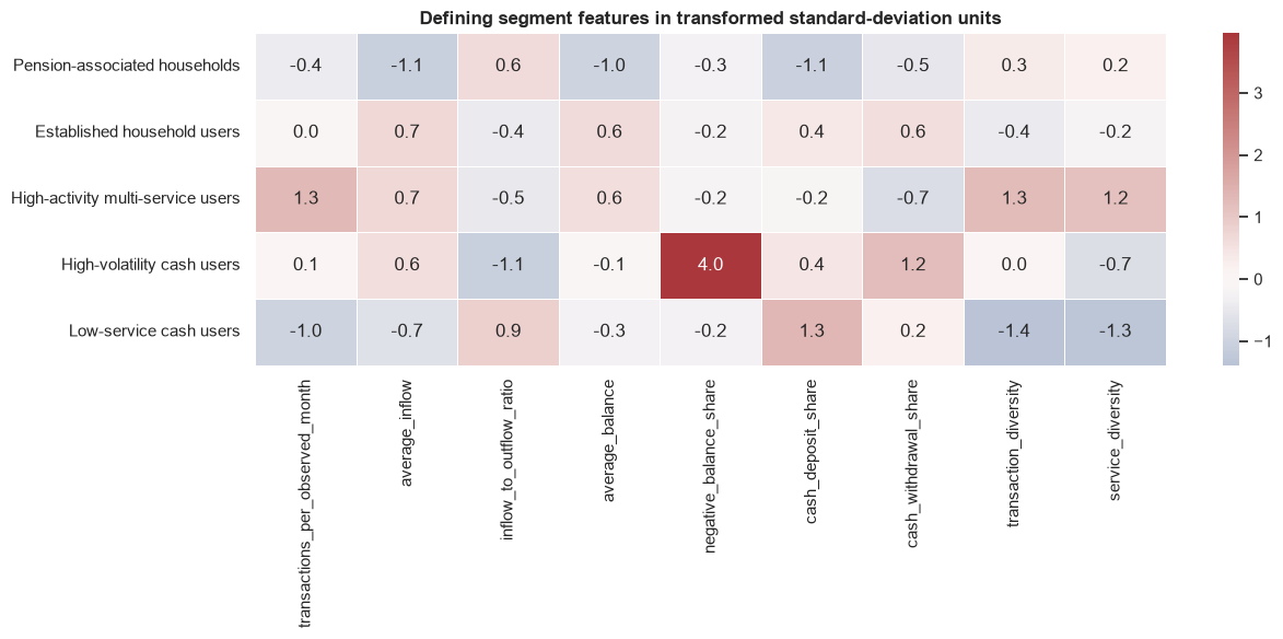
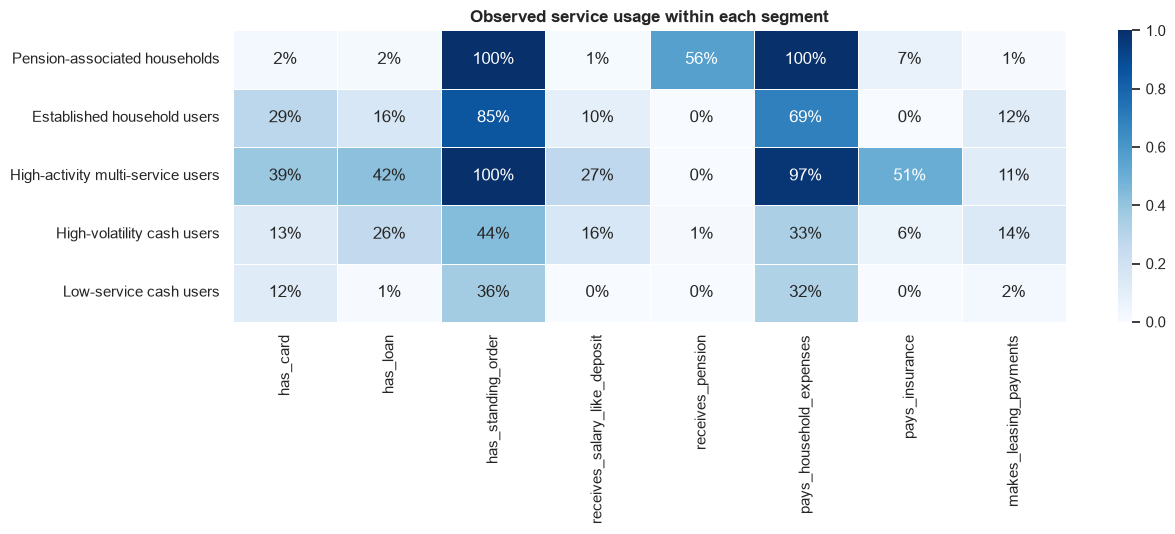
Numerical profiles use medians for continuous/skewed behaviors and account proportions for service indicators. “Defining features” are the three largest absolute K-means centroid coordinates in the transformed standardized space.
Code
profile_data = customer_features.copy()profile_data["segment_id"] = kmeans_labelsprofile_data["segment_name"] = segment_namescontinuous_profiles = ( profile_data.groupby(["segment_id", "segment_name"])[PROFILE_CONTINUOUS_FEATURES] .median() .add_prefix("median_"))service_profiles = ( profile_data.groupby(["segment_id", "segment_name"])[SERVICE_INDICATORS] .mean() .add_prefix("rate_"))population_profiles = ( profile_data.groupby(["segment_id", "segment_name"]) .size() .rename("population_size") .to_frame())population_profiles["population_share"] = population_profiles["population_size"] /len(profile_data)feature_display_names = {"transactions_per_observed_month": "transaction intensity","average_inflow": "average inflow","inflow_to_outflow_ratio": "inflow/outflow ratio","average_balance": "average balance","negative_balance_share": "negative-balance exposure","cash_deposit_share": "cash-deposit share","cash_withdrawal_share": "cash-withdrawal share","transaction_diversity": "transaction diversity","service_diversity": "service diversity",}def defining_feature_text(segment_id: int) ->str: centroid = pd.Series(kmeans_model.cluster_centers_[segment_id], index=MODEL_FEATURES) strongest = centroid.abs().nlargest(3).index descriptions = []for feature in strongest: direction ="high"if centroid[feature] >0else"low" descriptions.append(f"{direction}{feature_display_names[feature]} ({centroid[feature]:+.2f} SD)" )return"; ".join(descriptions)segment_narratives = {"Pension-associated households": {"transaction_patterns": "Lower-value recurring inflows, very low cash-deposit share, and regular household payments.","balance_characteristics": "Lowest typical balances and comparatively low balance volatility.","banking_service_usage": "Nearly universal standing orders and household payments; pension deposits are common; cards and loans are uncommon.","possible_business_relevance": "Investigate accessible servicing and reliable recurring-payment support.","limitations": "The pension flag is historical and not universal in this segment; it must not be treated as age, vulnerability, or suitability evidence.", },"Established household users": {"transaction_patterns": "Moderate activity with larger inflows and mixed cash usage.","balance_characteristics": "High typical balances with moderate volatility.","banking_service_usage": "Household payments and standing orders are common; cards and leasing appear more often than portfolio average.","possible_business_relevance": "Investigate everyday-service experience and channel support for established relationships.","limitations": "High balance and service use do not establish profitability, loyalty, or unmet product need.", },"High-activity multi-service users": {"transaction_patterns": "Highest transaction intensity and transaction diversity with relatively lower cash-withdrawal share.","balance_characteristics": "High typical balances with moderate volatility.","banking_service_usage": "Broadest service use; loans, cards, insurance, standing orders, and salary-like deposits are comparatively frequent.","possible_business_relevance": "Investigate service coordination and operational capacity for complex account activity.","limitations": "High activity is not evidence of customer value, credit suitability, or willingness to receive additional services.", },"High-volatility cash users": {"transaction_patterns": "High cash-withdrawal share and relatively high outflows.","balance_characteristics": "Highest balance volatility and the clearest negative-balance exposure.","banking_service_usage": "Fewer recurring services, although loans and leasing are present for some accounts.","possible_business_relevance": "Investigate aggregate cash-flow support and servicing friction without punitive treatment.","limitations": "Volatility and negative balances are valid financial behavior, not proof of distress, default, fraud, or misconduct.", },"Low-service cash users": {"transaction_patterns": "Lower activity and diversity with a high cash-deposit share.","balance_characteristics": "Mid-range typical balances and moderate volatility.","banking_service_usage": "Few observed services; loans, salary-like deposits, insurance, and leasing are rare.","possible_business_relevance": "Investigate voluntary onboarding, education, or simpler channel support.","limitations": "Low observed service use does not imply low engagement, unmet need, digital exclusion, or receptiveness to marketing.", },}segment_profiles = population_profiles.join(continuous_profiles).join(service_profiles).reset_index()segment_profiles["defining_features"] = segment_profiles["segment_id"].map(defining_feature_text)for narrative_column in ["transaction_patterns","balance_characteristics","banking_service_usage","possible_business_relevance","limitations",]: segment_profiles[narrative_column] = segment_profiles["segment_name"].map(lambda segment_name: segment_narratives[segment_name][narrative_column] )display( segment_profiles[ ["segment_name","population_size","population_share","defining_features","median_transactions_per_observed_month","median_average_inflow","median_average_balance","median_balance_std","median_service_diversity", ] ])
segment_name
population_size
population_share
defining_features
median_transactions_per_observed_month
median_average_inflow
median_average_balance
median_balance_std
median_service_diversity
0
Pension-associated households
1305
0.290000
low average inflow (-1.09 SD); low cash-deposi...
4.900000
2542.140625
20899.565217
5000.970702
3.0
1
Established household users
1519
0.337556
high average inflow (+0.71 SD); high average b...
5.538462
10793.585859
45623.111111
14253.370040
2.0
2
High-activity multi-service users
838
0.186222
high transaction intensity (+1.31 SD); high tr...
7.291078
11062.640341
45009.918542
14011.153640
4.0
3
High-volatility cash users
251
0.055778
high negative-balance exposure (+3.96 SD); hig...
5.500000
10677.592000
35546.471698
25030.567393
1.0
4
Low-service cash users
587
0.130444
low transaction diversity (-1.39 SD); high cas...
4.638298
3247.747475
30737.750000
10477.222205
0.0
Code
centroid_profile = pd.DataFrame( kmeans_model.cluster_centers_, index=[SEGMENT_NAME_MAP[index] for index inrange(SELECTED_K)], columns=MODEL_FEATURES,)fig, ax = plt.subplots(figsize=(13, 6))sns.heatmap( centroid_profile, cmap="vlag", center=0, annot=True, fmt=".1f", linewidths=0.4, ax=ax,)ax.set(title="Defining segment features in transformed standard-deviation units", xlabel="", ylabel="")fig.tight_layout()plt.show()service_rate_profile = segment_profiles.set_index("segment_name")[ ["rate_"+ feature for feature in SERVICE_INDICATORS]]service_rate_profile.columns = [column.removeprefix("rate_") for column in service_rate_profile.columns]fig, ax = plt.subplots(figsize=(13, 5.5))sns.heatmap( service_rate_profile, cmap="Blues", vmin=0, vmax=1, annot=True, fmt=".0%", linewidths=0.4, ax=ax,)ax.set(title="Observed service usage within each segment", xlabel="", ylabel="")fig.tight_layout()plt.show()
An outlier is an account that differs from a defined behavioral reference—not evidence of fraud, harm, or error. Four complementary signals are calculated:
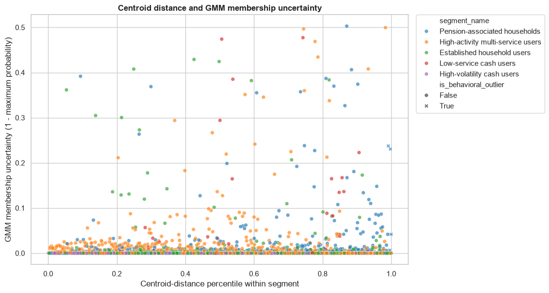
Centroid distance: distance from the assigned K-means centre, ranked within segment.
Low GMM membership: low maximum probability under the matched five-component GMM.
Robust within-segment deviation: largest median/MAD-based deviation across transformed model features, with IQR or standard-deviation fallback when MAD is zero.
Isolation Forest: model-independent nonlinear comparison using a 1% contamination setting.
An account is selected for case-study review only when at least two signals flag it. This consensus rule reduces dependence on any single geometric assumption.
The case-study table identifies why an account is unusual relative to its segment and shows the corresponding segment median. It does not establish an explanation. Investigation would require contemporaneous context, data-quality review, and appropriate authority; no account should receive adverse treatment from this analysis.
11. Persist and validate outputs
Artifact
Grain or type
Purpose
customer_segments.parquet
One row per account
Selected segment assignment and PCA coordinates
segment_profiles.parquet
One row per segment
Numeric profiles, interpretation, relevance, and limitations
behavioral_outliers.parquet
One row per account
Transparent outlier scores, flags, and consensus selection
clustering_evaluation.parquet
One row per algorithm and tested K
K-means and GMM model-selection evidence for the dashboard
Nine selected behaviors are transformed and scaled reproducibly; omitting skewness treatment produces an unstable tiny cluster.
The first two PCs explain about 63.4% of variance, while four PCs explain about 86.2%. PCA loadings support interpretable activity/breadth and financial-scale dimensions.
K-means with five segments provides the strongest tested combination of elbow behavior, silhouette, Davies-Bouldin score, cluster size, stability, and business interpretability.
The five segments contain 1,305 pension-associated households, 1,519 established household users, 838 high-activity multi-service users, 251 high-volatility cash users, and 587 low-service cash users.
GMM is stable but less separated at matched K. Its membership probabilities remain useful as a complementary uncertainty signal.
Sixteen accounts meet the conservative two-signal behavioral-outlier rule. They are analytical case studies, not suspicious accounts or fraud cases.
Segment names summarize dominant historical patterns and must not become permanent customer labels.
Next notebook:04_validation_and_insights.ipynb will validate segment usefulness and limitations, conduct the bounded supervised-learning case study, examine data-centric error patterns, and synthesize the final recommendations.