04 — Validation and Insights

Project: Transaction Intelligence: Customer Segmentation and Behavioral Analytics
Dataset: Berka / PKDD’99 Financial Dataset
Course alignment:

• Week 9 — Supervised Learning Techniques
• Week 10 — Data-Centric AI and Explainability
• Final project synthesis

This notebook checks the quality and limits of the full project. It includes a small loan-outcome case study to demonstrate supervised learning, reviews the data and earlier clustering results, explains the main outputs, and creates four simple tables for the dashboard.

The loan case study is not the main purpose of the project. It is not a lending system, a credit score, or a fraud model.

Notebook objectives

1. Build a loan-level dataset using only information available before each loan began.
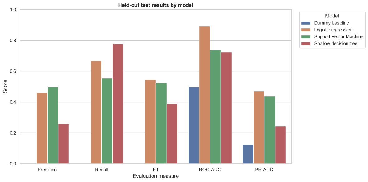
2. Compare a simple baseline, logistic regression, a Support Vector Machine, and a small decision tree.
3. Evaluate the models with measures that are useful when one outcome is uncommon.
4. Review missing data, coverage, time differences, regional representation, and model errors.
5. Recheck cluster stability and explain segments, PCA, and behavioral outliers in simple terms.
6. Bring the main findings together and create dashboard-ready tables.

1. Analytical contract

Loan case-study question

Among completed loans, can information known when a loan began help distinguish loans completed with and without repayment problems?

The unit of analysis is one completed loan. The target is:

• 0: completed without recorded repayment problems;
• 1: completed with recorded repayment problems.

Active loans are excluded because their final outcome is not yet known in this historical snapshot.

Safe-use rules

• Results are a course-method demonstration, not a recommendation to approve or reject credit.
• Transactions after the loan date are never used as inputs.
• Loan status, later payments, current segments, and outlier labels are not model inputs.
• Gender, age, and location are not used by the main model. They are kept only for limited quality checks.
• A model error or behavioral outlier is not evidence of fraud, wrongdoing, or poor character.
• The data are historical and cannot describe present-day customers or banking conditions.

Course content and small extensions

Part	Role in this notebook
Logistic regression, SVM, decision tree, confusion matrix, precision, recall, and F1	Week 9 course content
Data quality, bias, error analysis, reproducibility, and explanations	Week 10 course content
Dummy classifier	A simple comparison point: it predicts the most common outcome
Leakage audit	A safety check that keeps future information out of the model
ROC-AUC and PR-AUC	Extra summary measures; PR-AUC is especially helpful when problem loans are rare
Cluster stability, segment profiles, and PCA loadings	Week 8 results checked again here

2. Reproducible setup and required inputs

Notebooks 1–3 produced the clean data, behavior features, segments, and outlier results used here. This notebook reads those files instead of repeating the earlier work.

from pathlib import Path
import hashlib
import platform

import duckdb
import joblib
import matplotlib.pyplot as plt
import numpy as np
import pandas as pd
import seaborn as sns
import sklearn
from IPython.display import display
from sklearn.base import clone
from sklearn.cluster import KMeans
from sklearn.compose import ColumnTransformer
from sklearn.dummy import DummyClassifier
from sklearn.impute import SimpleImputer
from sklearn.linear_model import LogisticRegression
from sklearn.metrics import (
    ConfusionMatrixDisplay,
    accuracy_score,
    adjusted_rand_score,
    average_precision_score,
    confusion_matrix,
    f1_score,
    precision_score,
    recall_score,
    roc_auc_score,
)
from sklearn.model_selection import train_test_split
from sklearn.pipeline import Pipeline
from sklearn.preprocessing import OneHotEncoder, StandardScaler
from sklearn.svm import SVC
from sklearn.tree import DecisionTreeClassifier


def find_project_root(start: Path | None = None) -> Path:
    current = (start or Path.cwd()).resolve()
    for candidate in (current, *current.parents):
        if (candidate / "pyproject.toml").is_file():
            return candidate
    raise FileNotFoundError("Could not locate the project root containing pyproject.toml")


def sql_literal(path: Path) -> str:
    return "'" + str(path).replace("'", "''") + "'"


def short_sha256(path: Path) -> str:
    digest = hashlib.sha256()
    with path.open("rb") as file:
        for chunk in iter(lambda: file.read(1_048_576), b""):
            digest.update(chunk)
    return digest.hexdigest()[:12]


PROJECT_ROOT = find_project_root()
INTERIM_DIR = PROJECT_ROOT / "data" / "interim"
PROCESSED_DIR = PROJECT_ROOT / "data" / "processed"
MODELS_DIR = PROJECT_ROOT / "models"
FIGURES_DIR = PROJECT_ROOT / "reports" / "figures"

DATABASE_PATH = INTERIM_DIR / "berka.duckdb"
TRANSACTIONS_PATH = INTERIM_DIR / "transactions_clean.parquet"
LOANS_PATH = INTERIM_DIR / "loans_clean.parquet"
ACCOUNT_BASE_PATH = INTERIM_DIR / "account_analytical_base.parquet"
CUSTOMER_FEATURES_PATH = PROCESSED_DIR / "customer_behavior_features.parquet"
MONTHLY_ACTIVITY_PATH = PROCESSED_DIR / "monthly_banking_activity.parquet"
ASSOCIATION_RULES_PATH = PROCESSED_DIR / "service_association_rules.parquet"
CUSTOMER_SEGMENTS_PATH = PROCESSED_DIR / "customer_segments.parquet"
SEGMENT_PROFILES_PATH = PROCESSED_DIR / "segment_profiles.parquet"
BEHAVIORAL_OUTLIERS_PATH = PROCESSED_DIR / "behavioral_outliers.parquet"

PREPROCESSING_MODEL_PATH = MODELS_DIR / "preprocessing_pipeline.joblib"
PCA_MODEL_PATH = MODELS_DIR / "pca.joblib"
CLUSTERING_MODEL_PATH = MODELS_DIR / "clustering_model.joblib"

PROCESSED_DIR.mkdir(parents=True, exist_ok=True)
FIGURES_DIR.mkdir(parents=True, exist_ok=True)

RANDOM_STATE = 42
sns.set_theme(style="whitegrid", context="notebook")
plt.rcParams.update({"figure.figsize": (11, 5.5), "axes.titleweight": "bold"})

environment = pd.Series(
    {
        "Python": platform.python_version(),
        "DuckDB": duckdb.__version__,
        "pandas": pd.__version__,
        "scikit-learn": sklearn.__version__,
        "Random state": RANDOM_STATE,
        "Project root": ".",
    },
    name="value",
)
display(environment.to_frame())

	value
Python	3.14.6
DuckDB	1.5.5
pandas	3.0.5
scikit-learn	1.9.0
Random state	42
Project root	.

required_inputs = {
    "Local DuckDB database": DATABASE_PATH,
    "Clean transactions": TRANSACTIONS_PATH,
    "Clean loans": LOANS_PATH,
    "Account analytical base": ACCOUNT_BASE_PATH,
    "Customer behavior features": CUSTOMER_FEATURES_PATH,
    "Monthly banking activity": MONTHLY_ACTIVITY_PATH,
    "Service association rules": ASSOCIATION_RULES_PATH,
    "Customer segments": CUSTOMER_SEGMENTS_PATH,
    "Segment profiles": SEGMENT_PROFILES_PATH,
    "Behavioral outliers": BEHAVIORAL_OUTLIERS_PATH,
    "Segmentation preprocessor": PREPROCESSING_MODEL_PATH,
    "PCA model": PCA_MODEL_PATH,
    "Clustering model": CLUSTERING_MODEL_PATH,
}

input_status = pd.DataFrame(
    [
        {
            "input": name,
            "path": str(path.relative_to(PROJECT_ROOT)),
            "exists": path.is_file(),
            "size_mb": round(path.stat().st_size / 1_048_576, 3) if path.is_file() else None,
        }
        for name, path in required_inputs.items()
    ]
)
display(input_status)
assert input_status["exists"].all(), "Run Notebooks 1–3 before this notebook."

connection = duckdb.connect(str(DATABASE_PATH), read_only=True)

transactions_scan = "read_parquet(" + sql_literal(TRANSACTIONS_PATH) + ")"
loans_scan = "read_parquet(" + sql_literal(LOANS_PATH) + ")"
account_base_scan = "read_parquet(" + sql_literal(ACCOUNT_BASE_PATH) + ")"

customer_features = connection.execute(
    "SELECT * FROM read_parquet(" + sql_literal(CUSTOMER_FEATURES_PATH) + ") ORDER BY account_id"
).fetchdf()
monthly_activity = connection.execute(
    "SELECT * FROM read_parquet(" + sql_literal(MONTHLY_ACTIVITY_PATH) + ") ORDER BY month"
).fetchdf()
association_rules_data = connection.execute(
    "SELECT * FROM read_parquet(" + sql_literal(ASSOCIATION_RULES_PATH) + ")"
).fetchdf()
customer_segments = connection.execute(
    "SELECT * FROM read_parquet(" + sql_literal(CUSTOMER_SEGMENTS_PATH) + ") ORDER BY account_id"
).fetchdf()
segment_profiles = connection.execute(
    "SELECT * FROM read_parquet(" + sql_literal(SEGMENT_PROFILES_PATH) + ") ORDER BY segment_id"
).fetchdf()
behavioral_outliers = connection.execute(
    "SELECT * FROM read_parquet(" + sql_literal(BEHAVIORAL_OUTLIERS_PATH) + ") ORDER BY account_id"
).fetchdf()

assert len(customer_features) == customer_features["account_id"].nunique()
assert len(customer_segments) == customer_segments["account_id"].nunique()
assert len(segment_profiles) == customer_segments["segment_id"].nunique()
assert len(behavioral_outliers) == behavioral_outliers["account_id"].nunique()

input_versions = pd.DataFrame(
    [
        {
            "path": str(path.relative_to(PROJECT_ROOT)),
            "sha256_first_12": short_sha256(path),
        }
        for path in required_inputs.values()
    ]
)
display(input_versions)

	input	path	exists	size_mb
0	Local DuckDB database	data/interim/berka.duckdb	True	46.262
1	Clean transactions	data/interim/transactions_clean.parquet	True	7.636
2	Clean loans	data/interim/loans_clean.parquet	True	0.010
3	Account analytical base	data/interim/account_analytical_base.parquet	True	0.121
4	Customer behavior features	data/processed/customer_behavior_features.parquet	True	0.369
5	Monthly banking activity	data/processed/monthly_banking_activity.parquet	True	0.006
6	Service association rules	data/processed/service_association_rules.parquet	True	0.003
7	Customer segments	data/processed/customer_segments.parquet	True	0.079
8	Segment profiles	data/processed/segment_profiles.parquet	True	0.009
9	Behavioral outliers	data/processed/behavioral_outliers.parquet	True	0.216
10	Segmentation preprocessor	models/preprocessing_pipeline.joblib	True	0.002
11	PCA model	models/pca.joblib	True	0.002
12	Clustering model	models/clustering_model.joblib	True	0.018

	path	sha256_first_12
0	data/interim/berka.duckdb	d9bcd69bec26
1	data/interim/transactions_clean.parquet	607e811971e0
2	data/interim/loans_clean.parquet	78e38d6502f9
3	data/interim/account_analytical_base.parquet	355d1f93389b
4	data/processed/customer_behavior_features.parquet	8b65f2ccc981
5	data/processed/monthly_banking_activity.parquet	e95b6ee151eb
6	data/processed/service_association_rules.parquet	b055f55a49ad
7	data/processed/customer_segments.parquet	a3f2b24a983d
8	data/processed/segment_profiles.parquet	232af49fd0c2
9	data/processed/behavioral_outliers.parquet	cc8a99817b78
10	models/preprocessing_pipeline.joblib	a889bd29045a
11	models/pca.joblib	b38240afda0b
12	models/clustering_model.joblib	3f3a32d34602

3. Week 9 — Supervised Learning Techniques

Build the completed-loan study table

Every transaction feature below is calculated with this rule:

transaction date < loan start date

This is the feature-availability cutoff. In plain language, the model may only use facts that would already have been known when the loan began.

LOAN_MODEL_SQL = """
WITH completed_loans AS (
    SELECT *
    FROM {loans}
    WHERE is_completed
),
preloan_transactions AS (
    SELECT
        l.loan_id,
        COUNT(t.trans_id) AS preloan_transaction_count,
        COUNT(DISTINCT DATE_TRUNC('month', t.transaction_date)) AS preloan_active_months,
        MAX(t.transaction_date) AS latest_preloan_transaction_date,
        AVG(t.amount) FILTER (WHERE t.transaction_direction = 'inflow')
            AS preloan_average_inflow,
        AVG(t.amount) FILTER (WHERE t.transaction_direction = 'outflow')
            AS preloan_average_outflow,
        SUM(t.amount) FILTER (WHERE t.transaction_direction = 'inflow')
            AS preloan_total_inflow,
        SUM(t.amount) FILTER (WHERE t.transaction_direction = 'outflow')
            AS preloan_total_outflow,
        AVG(t.balance) AS preloan_average_balance,
        STDDEV_POP(t.balance) AS preloan_balance_std,
        MIN(t.balance) AS preloan_minimum_balance,
        AVG(CAST(t.balance < 0 AS INTEGER)) AS preloan_negative_balance_share,
        COUNT(DISTINCT COALESCE(t.operation, 'missing')) AS preloan_operation_diversity,
        AVG(CAST(t.operation = 'incoming_transfer' AS INTEGER))
            AS preloan_incoming_transfer_share
    FROM completed_loans AS l
    JOIN {transactions} AS t
      ON l.account_id = t.account_id
     AND t.transaction_date < l.loan_date
    GROUP BY l.loan_id
)
SELECT
    l.loan_id,
    l.account_id,
    l.loan_date,
    EXTRACT(YEAR FROM l.loan_date)::INTEGER AS loan_year,
    l.loan_amount,
    l.duration_months,
    CAST(l.monthly_payment AS DOUBLE) AS monthly_payment,
    CAST(l.completed_repayment_problem AS INTEGER) AS repayment_problem,
    b.account_open_date,
    b.statement_frequency,
    b.account_region,
    b.account_district_id,
    b.owner_gender,
    DATE_DIFF('year', b.owner_birth_date, l.loan_date) AS owner_age_at_loan,
    GREATEST(DATE_DIFF('month', b.account_open_date, l.loan_date) + 1, 1)
        AS account_age_months_at_loan,
    CAST(b.first_card_issued IS NOT NULL AND b.first_card_issued <= l.loan_date AS INTEGER)
        AS has_card_before_loan,
    p.latest_preloan_transaction_date,
    p.preloan_transaction_count,
    p.preloan_active_months,
    p.preloan_transaction_count
        / GREATEST(DATE_DIFF('month', b.account_open_date, l.loan_date) + 1, 1)::DOUBLE
        AS preloan_transactions_per_month,
    p.preloan_active_months
        / GREATEST(DATE_DIFF('month', b.account_open_date, l.loan_date) + 1, 1)::DOUBLE
        AS preloan_active_month_ratio,
    p.preloan_average_inflow,
    p.preloan_average_outflow,
    p.preloan_total_inflow / NULLIF(p.preloan_total_outflow, 0)
        AS preloan_inflow_to_outflow_ratio,
    p.preloan_average_balance,
    p.preloan_balance_std,
    p.preloan_minimum_balance,
    p.preloan_negative_balance_share,
    p.preloan_operation_diversity,
    p.preloan_incoming_transfer_share,
    CAST(l.monthly_payment AS DOUBLE) / NULLIF(p.preloan_average_inflow, 0)
        AS payment_to_average_inflow_ratio
FROM completed_loans AS l
JOIN {account_base} AS b USING (account_id)
JOIN preloan_transactions AS p USING (loan_id)
ORDER BY l.loan_date, l.loan_id
""".format(
    loans=loans_scan,
    transactions=transactions_scan,
    account_base=account_base_scan,
)

loan_model_data = connection.execute(LOAN_MODEL_SQL).fetchdf()

loan_cohort_check = pd.Series(
    {
        "Completed loans": len(loan_model_data),
        "Unique loan IDs": loan_model_data["loan_id"].nunique(),
        "Loans with a recorded problem": loan_model_data["repayment_problem"].sum(),
        "Loans without a recorded problem": (loan_model_data["repayment_problem"] == 0).sum(),
        "Missing targets": loan_model_data["repayment_problem"].isna().sum(),
        "Latest allowed transaction is before loan date": bool(
            (loan_model_data["latest_preloan_transaction_date"] < loan_model_data["loan_date"]).all()
        ),
    },
    name="value",
)
display(loan_cohort_check.to_frame())

assert len(loan_model_data) == loan_model_data["loan_id"].nunique()
assert loan_model_data["repayment_problem"].notna().all()
assert (loan_model_data["latest_preloan_transaction_date"] < loan_model_data["loan_date"]).all()

	value
Completed loans	234
Unique loan IDs	234
Loans with a recorded problem	31
Loans without a recorded problem	203
Missing targets	0
Latest allowed transaction is before loan date	True

Target balance

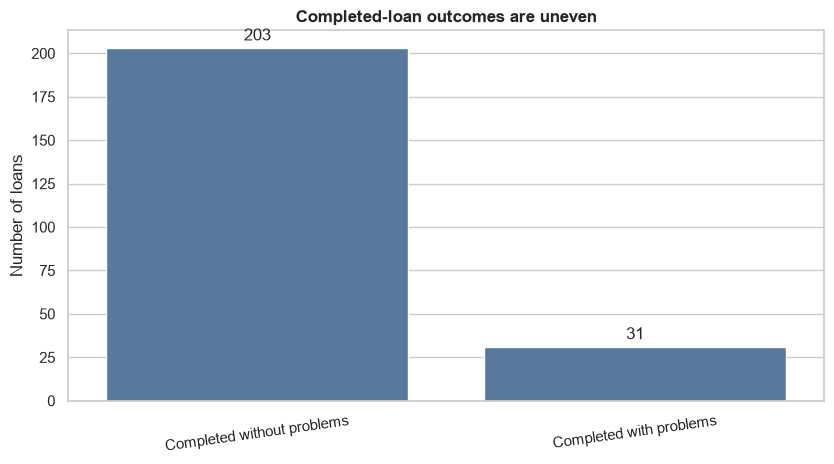
The two outcomes do not occur equally often. A model could look accurate by predicting the common outcome every time, while finding no problem loans at all. This is why the notebook reports precision, recall, F1, ROC-AUC, and PR-AUC instead of relying only on accuracy.

target_distribution = (
    loan_model_data["repayment_problem"]
    .map({0: "Completed without problems", 1: "Completed with problems"})
    .value_counts()
    .rename_axis("outcome")
    .reset_index(name="loans")
)
target_distribution["share_pct"] = 100 * target_distribution["loans"] / len(loan_model_data)
display(target_distribution)

fig, ax = plt.subplots(figsize=(8.5, 4.8))
sns.barplot(data=target_distribution, x="outcome", y="loans", color="#4C78A8", ax=ax)
for container in ax.containers:
    ax.bar_label(container, padding=3)
ax.set(title="Completed-loan outcomes are uneven", xlabel="", ylabel="Number of loans")
ax.tick_params(axis="x", rotation=8)
fig.tight_layout()
fig.savefig(FIGURES_DIR / "loan_target_distribution.png", dpi=160, bbox_inches="tight")
plt.show()

	outcome	loans	share_pct
0	Completed without problems	203	86.752137
1	Completed with problems	31	13.247863

Leakage audit and feature choices

Data leakage means giving the model information that would not have been available at the time of the decision. That can make results look much better than they really are.

Information	Use	Reason
Loan amount and planned duration	Model input	Known when the loan begins
Transactions before the loan date	Model input	Available history only
Statement frequency	Model input	Existing account setting
Loan status or later loan payments	Excluded	These reveal or follow the outcome
Transactions on or after the loan date	Excluded	Future information
Full-history customer features from Notebook 2	Excluded	They include activity after many loan dates
Segment and outlier labels	Excluded	They use the full historical observation window
Standing orders	Excluded	The source table has no start date, so availability cannot be proven
Gender, age, district, and region	Audit only	Not needed for the main prediction and sensitive to misuse
Card indicator	Sensitivity check only	Few completed-loan accounts had a card before the loan

The primary model uses a compact set of loan terms and earlier account behavior. Monthly payment is not used by itself because it is already determined by loan amount and duration. It is used only in a ratio that compares the planned payment with earlier average inflow.

LOAN_TERM_FEATURES = [
    "loan_amount",
    "duration_months",
]

PRELOAN_BEHAVIOR_FEATURES = [
    "account_age_months_at_loan",
    "preloan_transactions_per_month",
    "preloan_active_month_ratio",
    "preloan_average_inflow",
    "preloan_average_outflow",
    "preloan_inflow_to_outflow_ratio",
    "preloan_average_balance",
    "preloan_negative_balance_share",
    "preloan_operation_diversity",
    "preloan_incoming_transfer_share",
    "payment_to_average_inflow_ratio",
]

PRIMARY_NUMERIC_FEATURES = LOAN_TERM_FEATURES + PRELOAN_BEHAVIOR_FEATURES
PRIMARY_CATEGORICAL_FEATURES = ["statement_frequency"]
PRIMARY_FEATURES = PRIMARY_NUMERIC_FEATURES + PRIMARY_CATEGORICAL_FEATURES
TARGET = "repayment_problem"

feature_guide = pd.DataFrame(
    [
        ("Loan terms", "Loan amount and planned duration", "Known at the start"),
        ("Account history", "Months since the account opened", "Shows how much history exists"),
        ("Activity", "Transactions and active months", "Describes earlier account use"),
        ("Cash flow", "Average inflow, outflow, and their ratio", "Describes money moving in and out"),
        ("Balance", "Average balance and share of negative balances", "Describes earlier balance condition"),
        ("Channel mix", "Operation variety and incoming-transfer share", "Describes how the account was used"),
        ("Payment pressure", "Planned payment divided by earlier average inflow", "Compares the payment with earlier inflow"),
        ("Account setting", "Statement frequency", "A simple existing service setting"),
    ],
    columns=["group", "included information", "plain-language purpose"],
)
display(feature_guide)

	group	included information	plain-language purpose
0	Loan terms	Loan amount and planned duration	Known at the start
1	Account history	Months since the account opened	Shows how much history exists
2	Activity	Transactions and active months	Describes earlier account use
3	Cash flow	Average inflow, outflow, and their ratio	Describes money moving in and out
4	Balance	Average balance and share of negative balances	Describes earlier balance condition
5	Channel mix	Operation variety and incoming-transfer share	Describes how the account was used
6	Payment pressure	Planned payment divided by earlier average inflow	Compares the payment with earlier inflow
7	Account setting	Statement frequency	A simple existing service setting

Train/test split and preparation

The data are split once into:

• 70% training data: used to fit the models;
• 30% test data: kept aside until evaluation.

The split keeps roughly the same outcome share in both parts. This is called a stratified split. A random split is used because the completed-loan sample is small. The result measures performance on held-out loans from this historical sample; it does not prove performance on future loans.

Numeric values are filled with the training median when needed and then placed on a comparable scale. Statement frequency is converted into indicator columns. All preparation steps are fitted on the training data only.

X = loan_model_data[PRIMARY_FEATURES].copy()
y = loan_model_data[TARGET].astype(int)

X_train, X_test, y_train, y_test = train_test_split(
    X,
    y,
    test_size=0.30,
    random_state=RANDOM_STATE,
    stratify=y,
)

split_summary = pd.DataFrame(
    [
        {
            "split": "Training",
            "loans": len(y_train),
            "problem_loans": int(y_train.sum()),
            "problem_rate_pct": 100 * y_train.mean(),
        },
        {
            "split": "Test",
            "loans": len(y_test),
            "problem_loans": int(y_test.sum()),
            "problem_rate_pct": 100 * y_test.mean(),
        },
    ]
)
display(split_summary.round(2))


def make_preprocessor(numeric_features, categorical_features):
    steps = []
    if numeric_features:
        steps.append(
            (
                "numeric",
                Pipeline(
                    steps=[
                        ("fill_missing", SimpleImputer(strategy="median")),
                        ("scale", StandardScaler()),
                    ]
                ),
                numeric_features,
            )
        )
    if categorical_features:
        steps.append(
            (
                "categorical",
                OneHotEncoder(handle_unknown="ignore"),
                categorical_features,
            )
        )
    return ColumnTransformer(steps)


primary_preprocessor = make_preprocessor(
    PRIMARY_NUMERIC_FEATURES,
    PRIMARY_CATEGORICAL_FEATURES,
)

	split	loans	problem_loans	problem_rate_pct
0	Training	163	22	13.50
1	Test	71	9	12.68

Model comparison

Model	Simple description
Dummy classifier	Always follows the most common training outcome; it is the minimum comparison point
Logistic regression	Learns a weighted combination of the inputs and is easy to explain
Support Vector Machine (SVM)	Finds a flexible boundary between the two outcomes
Shallow decision tree	Uses a small set of yes/no splits; depth is limited to reduce overfitting

The three fitted models use balanced class weights. This asks them to pay more attention to the uncommon problem-loan class. It does not create new observations.

model_definitions = {
    "Dummy baseline": DummyClassifier(strategy="prior"),
    "Logistic regression": LogisticRegression(
        max_iter=2_000,
        class_weight="balanced",
        random_state=RANDOM_STATE,
    ),
    "Support Vector Machine": SVC(
        kernel="rbf",
        class_weight="balanced",
    ),
    "Shallow decision tree": DecisionTreeClassifier(
        max_depth=3,
        min_samples_leaf=10,
        class_weight="balanced",
        random_state=RANDOM_STATE,
    ),
}

fitted_models = {}
prediction_store = {}
evaluation_rows = []

for model_name, estimator in model_definitions.items():
    pipeline = Pipeline(
        steps=[
            ("preprocessing", clone(primary_preprocessor)),
            ("model", estimator),
        ]
    )
    pipeline.fit(X_train, y_train)
    predicted = pipeline.predict(X_test)
    if hasattr(pipeline, "predict_proba"):
        score = pipeline.predict_proba(X_test)[:, 1]
    else:
        score = pipeline.decision_function(X_test)

    fitted_models[model_name] = pipeline
    prediction_store[model_name] = {"predicted": predicted, "score": score}
    evaluation_rows.append(
        {
            "model": model_name,
            "accuracy": accuracy_score(y_test, predicted),
            "precision": precision_score(y_test, predicted, zero_division=0),
            "recall": recall_score(y_test, predicted, zero_division=0),
            "f1": f1_score(y_test, predicted, zero_division=0),
            "roc_auc": roc_auc_score(y_test, score),
            "pr_auc": average_precision_score(y_test, score),
            "predicted_problem_loans": int(predicted.sum()),
        }
    )

model_evaluation = pd.DataFrame(evaluation_rows)
display(model_evaluation.round(3))

	model	accuracy	precision	recall	f1	roc_auc	pr_auc	predicted_problem_loans
0	Dummy baseline	0.873	0.000	0.000	0.000	0.500	0.127	0
1	Logistic regression	0.859	0.462	0.667	0.545	0.892	0.471	13
2	Support Vector Machine	0.873	0.500	0.556	0.526	0.738	0.440	10
3	Shallow decision tree	0.690	0.259	0.778	0.389	0.723	0.245	27

metric_columns = ["precision", "recall", "f1", "roc_auc", "pr_auc"]
model_plot_data = model_evaluation.melt(
    id_vars="model",
    value_vars=metric_columns,
    var_name="measure",
    value_name="score",
)
model_plot_data["measure"] = model_plot_data["measure"].map(
    {
        "precision": "Precision",
        "recall": "Recall",
        "f1": "F1",
        "roc_auc": "ROC-AUC",
        "pr_auc": "PR-AUC",
    }
)

fig, ax = plt.subplots(figsize=(12, 6))
sns.barplot(data=model_plot_data, x="measure", y="score", hue="model", ax=ax)
ax.set(
    title="Held-out test results by model",
    xlabel="Evaluation measure",
    ylabel="Score",
    ylim=(0, 1),
)
ax.legend(title="Model", bbox_to_anchor=(1.02, 1), loc="upper left")
fig.tight_layout()
fig.savefig(FIGURES_DIR / "loan_model_comparison.png", dpi=160, bbox_inches="tight")
plt.show()

How to read the measures

• Precision: when the model flags a problem, how often is it correct?
• Recall: of the recorded problem loans, how many does the model find?
• F1: one score that balances precision and recall.
• ROC-AUC: how well the model generally ranks problem loans above non-problem loans across many cutoffs.
• PR-AUC: how well precision and recall work together across many cutoffs. It is useful here because problem loans are uncommon.

Logistic regression is kept as the main case-study model because it gives the best overall balance in this fixed comparison and its coefficients can be explained directly. The test set contains very few problem loans, so small changes in predictions can move these scores substantially.

SELECTED_LOAN_MODEL = "Logistic regression"
selected_predictions = prediction_store[SELECTED_LOAN_MODEL]["predicted"]
selected_scores = prediction_store[SELECTED_LOAN_MODEL]["score"]

fig, ax = plt.subplots(figsize=(6.8, 5.6))
ConfusionMatrixDisplay.from_predictions(
    y_test,
    selected_predictions,
    display_labels=["No recorded problem", "Recorded problem"],
    cmap="Blues",
    colorbar=False,
    ax=ax,
)
ax.set_title("Logistic-regression test predictions")
fig.tight_layout()
fig.savefig(FIGURES_DIR / "loan_logistic_confusion_matrix.png", dpi=160, bbox_inches="tight")
plt.show()

tn, fp, fn, tp = confusion_matrix(y_test, selected_predictions).ravel()
confusion_summary = pd.Series(
    {
        "Correct non-problem predictions": tn,
        "False alarms": fp,
        "Missed problem loans": fn,
        "Correct problem predictions": tp,
    },
    name="loans",
)
display(confusion_summary.to_frame())

	loans
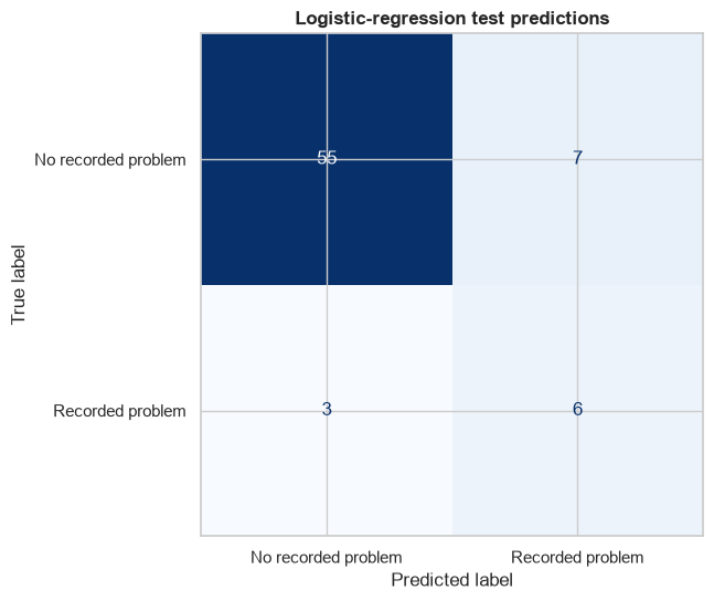
Correct non-problem predictions	55
False alarms	7
Missed problem loans	3
Correct problem predictions	6

Error review

A confusion matrix counts correct and incorrect predictions. The next table looks at the actual test cases behind those counts. This can show where the model struggles, but it cannot prove why a repayment problem happened.

test_results = loan_model_data.loc[X_test.index].copy()
test_results["actual_problem"] = y_test
test_results["predicted_problem"] = selected_predictions
test_results["model_score"] = selected_scores
test_results["result_type"] = np.select(
    [
        (test_results["actual_problem"] == 0) & (test_results["predicted_problem"] == 0),
        (test_results["actual_problem"] == 0) & (test_results["predicted_problem"] == 1),
        (test_results["actual_problem"] == 1) & (test_results["predicted_problem"] == 0),
        (test_results["actual_problem"] == 1) & (test_results["predicted_problem"] == 1),
    ],
    ["correct non-problem", "false alarm", "missed problem", "correct problem"],
    default="unknown",
)

error_counts = test_results["result_type"].value_counts().rename_axis("result_type").reset_index(name="loans")
display(error_counts)

error_feature_summary = (
    test_results.groupby("result_type")
    .agg(
        loans=("loan_id", "size"),
        median_loan_amount=("loan_amount", "median"),
        median_payment_to_inflow=("payment_to_average_inflow_ratio", "median"),
        median_preloan_balance=("preloan_average_balance", "median"),
        median_preloan_transactions_per_month=("preloan_transactions_per_month", "median"),
    )
    .reset_index()
)
display(error_feature_summary.round(2))

error_case_view = test_results.loc[
        test_results["actual_problem"] != test_results["predicted_problem"],
        [
            "loan_id",
            "loan_date",
            "actual_problem",
            "predicted_problem",
            "model_score",
            "loan_amount",
            "payment_to_average_inflow_ratio",
            "preloan_average_balance",
            "account_region",
        ],
    ].sort_values("model_score", ascending=False)
numeric_error_columns = [
    "model_score",
    "loan_amount",
    "payment_to_average_inflow_ratio",
    "preloan_average_balance",
]
error_case_view[numeric_error_columns] = error_case_view[numeric_error_columns].round(3)
display(error_case_view)

	result_type	loans
0	correct non-problem	55
1	false alarm	7
2	correct problem	6
3	missed problem	3

	result_type	loans	median_loan_amount	median_payment_to_inflow	median_preloan_balance	median_preloan_transactions_per_month
0	correct non-problem	55	74040.0	0.31	42291.30	5.36
1	correct problem	6	140268.0	0.46	34536.50	3.43
2	false alarm	7	134784.0	0.64	44131.23	5.25
3	missed problem	3	75624.0	0.27	50010.00	3.29

	loan_id	loan_date	actual_problem	predicted_problem	model_score	loan_amount	payment_to_average_inflow_ratio	preloan_average_balance	account_region
9	5997	1993-11-04	0	1	0.824	117024	0.371	44131.231	south Bohemia
69	6841	1994-08-07	0	1	0.669	172080	0.335	60744.119	central Bohemia
117	6694	1995-03-19	0	1	0.638	134784	0.637	44005.164	north Moravia
156	6589	1996-01-01	0	1	0.636	189696	0.424	54136.966	south Bohemia
105	5739	1995-01-02	0	1	0.635	76380	1.385	26122.733	Prague
179	5375	1996-10-03	0	1	0.635	101520	1.379	26449.289	Prague
88	6808	1994-10-12	0	1	0.530	227880	0.780	45134.783	south Moravia
65	5395	1994-07-30	1	0	0.468	299088	0.470	51992.944	north Moravia
19	7097	1993-12-23	1	0	0.461	75624	0.270	50010.000	south Moravia
159	6027	1996-02-10	1	0	0.426	61656	0.184	44763.500	central Bohemia

Logistic-regression explanation

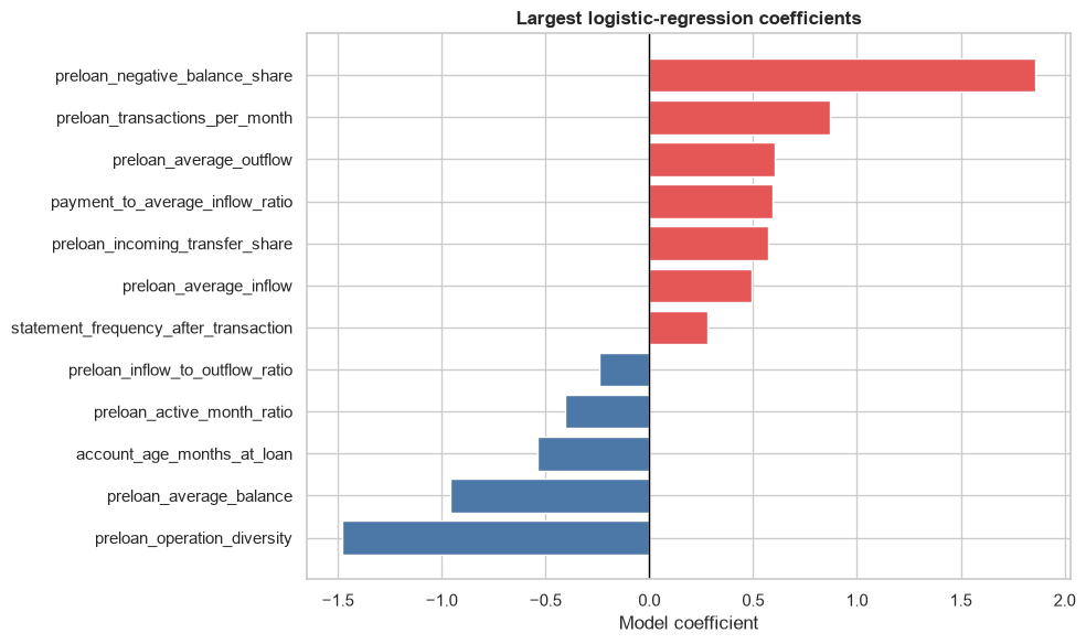
A positive coefficient moves the model toward the “recorded problem” outcome. A negative coefficient moves it away. Larger absolute values have more influence inside this fitted model.

Coefficients show model associations after scaling; they do not show cause. Correlated inputs can also share or move influence between them.

logistic_pipeline = fitted_models[SELECTED_LOAN_MODEL]
transformed_feature_names = logistic_pipeline.named_steps["preprocessing"].get_feature_names_out()
coefficient_values = logistic_pipeline.named_steps["model"].coef_[0]

coefficient_table = pd.DataFrame(
    {
        "feature": transformed_feature_names,
        "coefficient": coefficient_values,
        "absolute_coefficient": np.abs(coefficient_values),
    }
).sort_values("absolute_coefficient", ascending=False)
coefficient_table["feature"] = (
    coefficient_table["feature"]
    .str.replace("numeric__", "", regex=False)
    .str.replace("categorical__", "", regex=False)
)
display(coefficient_table.head(12).round(3))

top_coefficients = coefficient_table.head(12).sort_values("coefficient")
fig, ax = plt.subplots(figsize=(10, 6))
colors = np.where(top_coefficients["coefficient"] >= 0, "#E45756", "#4C78A8")
ax.barh(top_coefficients["feature"], top_coefficients["coefficient"], color=colors)
ax.axvline(0, color="black", linewidth=1)
ax.set(title="Largest logistic-regression coefficients", xlabel="Model coefficient", ylabel="")
fig.tight_layout()
plt.show()

	feature	coefficient	absolute_coefficient
9	preloan_negative_balance_share	1.861	1.861
10	preloan_operation_diversity	-1.481	1.481
8	preloan_average_balance	-0.956	0.956
3	preloan_transactions_per_month	0.871	0.871
6	preloan_average_outflow	0.603	0.603
12	payment_to_average_inflow_ratio	0.595	0.595
11	preloan_incoming_transfer_share	0.572	0.572
2	account_age_months_at_loan	-0.541	0.541
5	preloan_average_inflow	0.493	0.493
4	preloan_active_month_ratio	-0.403	0.403
13	statement_frequency_after_transaction	0.281	0.281
7	preloan_inflow_to_outflow_ratio	-0.239	0.239

Why SHAP is not added: logistic-regression coefficients already give a clear explanation for this small demonstration. Adding another explanation tool would make the notebook longer without changing the main conclusion. SHAP would be useful later if a more complex final model needed individual explanations.

4. Week 10 — Data-Centric AI and Explainability

Data-centric AI asks whether the data are suitable, complete enough, representative enough, and reproducible. Better modelling cannot repair a poorly defined target or missing historical coverage.

Data quality before and after preparation

“Before” refers to the source-style loan table in the local DuckDB snapshot. “After” refers to the cleaned loan table from Notebook 1 and the completed-loan study table built above.

raw_loan_quality = connection.execute(
    """
    SELECT
        COUNT(*) AS rows,
        COUNT(DISTINCT loan_id) AS unique_loan_ids,
        COUNT(*) FILTER (
            WHERE loan_id IS NULL OR account_id IS NULL OR date IS NULL
               OR amount IS NULL OR duration IS NULL OR payments IS NULL OR status IS NULL
        ) AS rows_missing_required_values,
        COUNT(*) FILTER (WHERE status IN ('A', 'B', 'C', 'D')) AS recognized_status_codes
    FROM loan
    """
).fetchdf().iloc[0]

clean_loan_quality = connection.execute(
    """
    SELECT
        COUNT(*) AS rows,
        COUNT(DISTINCT loan_id) AS unique_loan_ids,
        COUNT(*) FILTER (
            WHERE loan_id IS NULL OR account_id IS NULL OR loan_date IS NULL
               OR loan_amount IS NULL OR duration_months IS NULL
               OR monthly_payment IS NULL OR loan_status IS NULL
        ) AS rows_missing_required_values,
        COUNT(*) FILTER (WHERE loan_status IS NOT NULL) AS readable_status_labels,
        COUNT(*) FILTER (WHERE is_completed AND completed_repayment_problem IS NOT NULL)
            AS completed_targets_available
    FROM read_parquet(""" + sql_literal(LOANS_PATH) + ")"
).fetchdf().iloc[0]

data_quality_comparison = pd.DataFrame(
    [
        {
            "check": "Rows retained",
            "source": int(raw_loan_quality["rows"]),
            "prepared": int(clean_loan_quality["rows"]),
            "meaning": "Cleaning did not silently remove loans",
        },
        {
            "check": "Unique loan IDs",
            "source": int(raw_loan_quality["unique_loan_ids"]),
            "prepared": int(clean_loan_quality["unique_loan_ids"]),
            "meaning": "One ID still identifies one loan",
        },
        {
            "check": "Rows missing required values",
            "source": int(raw_loan_quality["rows_missing_required_values"]),
            "prepared": int(clean_loan_quality["rows_missing_required_values"]),
            "meaning": "Core loan fields are complete",
        },
        {
            "check": "Recognized or readable statuses",
            "source": int(raw_loan_quality["recognized_status_codes"]),
            "prepared": int(clean_loan_quality["readable_status_labels"]),
            "meaning": "All four source codes have clear labels",
        },
        {
            "check": "Completed targets available",
            "source": "Not present",
            "prepared": int(clean_loan_quality["completed_targets_available"]),
            "meaning": "The target is defined only for completed loans",
        },
    ]
)
display(data_quality_comparison)

	check	source	prepared	meaning
0	Rows retained	682	682	Cleaning did not silently remove loans
1	Unique loan IDs	682	682	One ID still identifies one loan
2	Rows missing required values	0	0	Core loan fields are complete
3	Recognized or readable statuses	682	682	All four source codes have clear labels
4	Completed targets available	Not present	234	The target is defined only for completed loans

Missing values and coverage gaps

Missing values are not all the same. Here, two completed-loan accounts had no earlier outflow, so their earlier average outflow and inflow-to-outflow ratio are missing. The model fills these numeric values with the training median. No target is filled or guessed.

Coverage is a larger concern than those two missing values: only a small share of all accounts has a completed loan, and recorded problem loans are rarer still.

feature_missingness = (
    loan_model_data[PRIMARY_FEATURES]
    .isna()
    .sum()
    .rename("missing_values")
    .to_frame()
)
feature_missingness["missing_share_pct"] = 100 * feature_missingness["missing_values"] / len(loan_model_data)
display(feature_missingness.query("missing_values > 0").round(2))

portfolio_counts = connection.execute(
    "SELECT COUNT(*) AS accounts FROM " + account_base_scan
).fetchdf().iloc[0]
loan_counts = connection.execute(
    """
    SELECT
        COUNT(*) AS all_loans,
        COUNT(DISTINCT account_id) AS accounts_with_loans,
        COUNT(*) FILTER (WHERE is_completed) AS completed_loans,
        COUNT(*) FILTER (WHERE completed_repayment_problem) AS completed_problem_loans
    FROM read_parquet(""" + sql_literal(LOANS_PATH) + ")"
).fetchdf().iloc[0]

coverage_table = pd.DataFrame(
    [
        ("All accounts", int(portfolio_counts["accounts"]), "Full account-level project coverage"),
        ("Accounts with any loan", int(loan_counts["accounts_with_loans"]), "Only these accounts appear in the loan table"),
        ("Completed loans", int(loan_counts["completed_loans"]), "Only these have a final outcome for this target"),
        ("Completed loans with recorded problems", int(loan_counts["completed_problem_loans"]), "Uncommon positive class"),
    ],
    columns=["group", "count", "meaning"],
)
coverage_table["share_of_all_accounts_pct"] = 100 * coverage_table["count"] / int(portfolio_counts["accounts"])
display(coverage_table.round(2))

	missing_values	missing_share_pct
preloan_average_outflow	2	0.85
preloan_inflow_to_outflow_ratio	2	0.85

	group	count	meaning	share_of_all_accounts_pct
0	All accounts	4500	Full account-level project coverage	100.00
1	Accounts with any loan	682	Only these accounts appear in the loan table	15.16
2	Completed loans	234	Only these have a final outcome for this target	5.20
3	Completed loans with recorded problems	31	Uncommon positive class	0.69

Historical and time differences

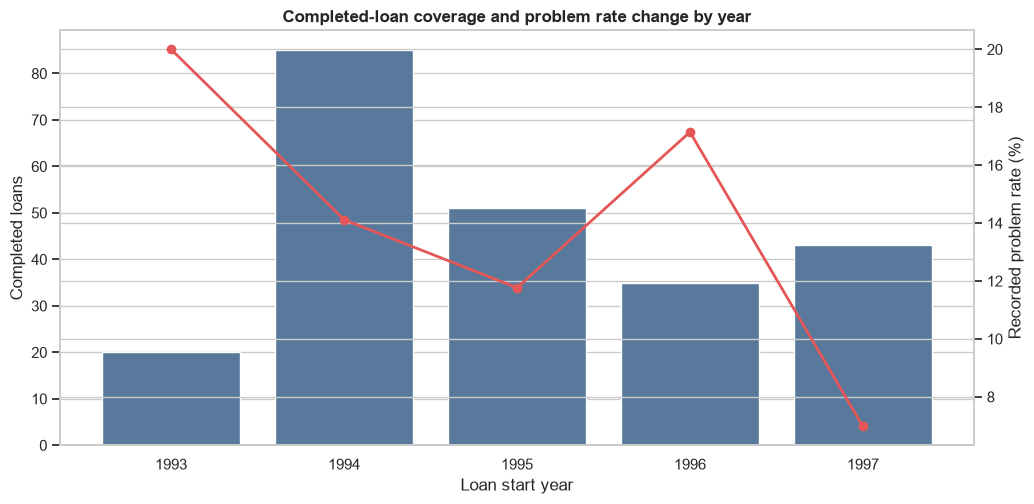
The data cover a short period in the 1990s. The number of completed loans and the recorded problem rate change by year. These differences may reflect changing customers, changing bank processes, or simple variation from small yearly counts.

loan_year_summary = (
    loan_model_data.groupby("loan_year")
    .agg(
        completed_loans=("loan_id", "size"),
        problem_loans=("repayment_problem", "sum"),
        problem_rate=("repayment_problem", "mean"),
    )
    .reset_index()
)
display(loan_year_summary.round(3))

fig, ax_count = plt.subplots(figsize=(10.5, 5.2))
sns.barplot(data=loan_year_summary, x="loan_year", y="completed_loans", color="#4C78A8", ax=ax_count)
ax_count.set(xlabel="Loan start year", ylabel="Completed loans", title="Completed-loan coverage and problem rate change by year")

ax_rate = ax_count.twinx()
ax_rate.plot(
    range(len(loan_year_summary)),
    100 * loan_year_summary["problem_rate"],
    color="#E45756",
    marker="o",
    linewidth=2,
)
ax_rate.set_ylabel("Recorded problem rate (%)")
fig.tight_layout()
fig.savefig(FIGURES_DIR / "loan_outcomes_by_year.png", dpi=160, bbox_inches="tight")
plt.show()

	loan_year	completed_loans	problem_loans	problem_rate
0	1993	20	4	0.200
1	1994	85	12	0.141
2	1995	51	6	0.118
3	1996	35	6	0.171
4	1997	43	3	0.070

Regional representation and error checks

Districts are too small for reliable district-by-district model conclusions, so the audit uses the eight broader regions. The table shows coverage and test errors. A high or low rate in a small group is a warning to investigate, not proof of bias or fairness.

region_coverage = (
    loan_model_data.groupby("account_region")
    .agg(
        completed_loans=("loan_id", "size"),
        problem_loans=("repayment_problem", "sum"),
        problem_rate=("repayment_problem", "mean"),
        represented_districts=("account_district_id", "nunique"),
    )
    .reset_index()
)

region_test_errors = (
    test_results.assign(is_error=test_results["actual_problem"] != test_results["predicted_problem"])
    .groupby("account_region")
    .agg(
        test_loans=("loan_id", "size"),
        test_errors=("is_error", "sum"),
        test_error_rate=("is_error", "mean"),
    )
    .reset_index()
)

region_audit = region_coverage.merge(region_test_errors, on="account_region", how="left")
display(region_audit.sort_values("completed_loans", ascending=False).round(3))

	account_region	completed_loans	problem_loans	problem_rate	represented_districts	test_loans	test_errors	test_error_rate
4	north Moravia	41	6	0.146	10	11	2	0.182
6	south Moravia	41	6	0.146	13	11	2	0.182
0	Prague	37	3	0.081	1	19	2	0.105
1	central Bohemia	31	5	0.161	11	8	2	0.250
5	south Bohemia	23	5	0.217	8	5	2	0.400
7	west Bohemia	22	5	0.227	8	9	0	0.000
3	north Bohemia	20	1	0.050	8	2	0	0.000
2	east Bohemia	19	0	0.000	11	6	0	0.000

Feature sensitivity

A sensitivity check asks whether the conclusion changes when the input set changes. The same logistic-regression method and the same train/test rows are used three times:

1. loan terms only;
2. loan terms plus earlier account behavior;
3. the same inputs plus region and the rare pre-loan card indicator.

This is not a search for the highest possible score. It checks whether extra information adds clear value.

feature_variants = {
    "Loan terms only": (LOAN_TERM_FEATURES, []),
    "Terms + pre-loan behavior": (
        LOAN_TERM_FEATURES + PRELOAN_BEHAVIOR_FEATURES,
        ["statement_frequency"],
    ),
    "Add region and card": (
        LOAN_TERM_FEATURES + PRELOAN_BEHAVIOR_FEATURES,
        ["statement_frequency", "account_region", "has_card_before_loan"],
    ),
}

feature_sensitivity_rows = []
for variant_name, (numeric_features, categorical_features) in feature_variants.items():
    variant_features = numeric_features + categorical_features
    variant_pipeline = Pipeline(
        steps=[
            ("preprocessing", make_preprocessor(numeric_features, categorical_features)),
            (
                "model",
                LogisticRegression(
                    max_iter=2_000,
                    class_weight="balanced",
                    random_state=RANDOM_STATE,
                ),
            ),
        ]
    )
    variant_pipeline.fit(
        loan_model_data.loc[X_train.index, variant_features],
        y_train,
    )
    variant_prediction = variant_pipeline.predict(
        loan_model_data.loc[X_test.index, variant_features]
    )
    variant_score = variant_pipeline.predict_proba(
        loan_model_data.loc[X_test.index, variant_features]
    )[:, 1]
    feature_sensitivity_rows.append(
        {
            "feature_set": variant_name,
            "input_columns": len(variant_features),
            "precision": precision_score(y_test, variant_prediction, zero_division=0),
            "recall": recall_score(y_test, variant_prediction, zero_division=0),
            "f1": f1_score(y_test, variant_prediction, zero_division=0),
            "roc_auc": roc_auc_score(y_test, variant_score),
            "pr_auc": average_precision_score(y_test, variant_score),
        }
    )

feature_sensitivity = pd.DataFrame(feature_sensitivity_rows)
display(feature_sensitivity.round(3))

	feature_set	input_columns	precision	recall	f1	roc_auc	pr_auc
0	Loan terms only	2	0.200	0.444	0.276	0.610	0.348
1	Terms + pre-loan behavior	14	0.462	0.667	0.545	0.892	0.471
2	Add region and card	16	0.444	0.444	0.444	0.900	0.511

Earlier account behavior adds useful information in this fixed split. Adding region and the rare card indicator lowers F1, while the two ranking measures rise slightly. With so few problem loans, these small differences are not strong evidence that the extra inputs help. The simpler “terms + pre-loan behavior” set is therefore kept, and location stays out of the main model.

Cluster stability check

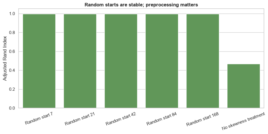
Notebook 3 selected five K-means segments. Here, the saved preparation steps are reused and K-means is fitted again with several random starting points.

The Adjusted Rand Index (ARI) compares two sets of segment assignments. A value near 1 means the assignments are almost the same. This checks repeatability; it does not prove that the segments are natural or permanent customer types.

saved_segmentation_preprocessor = joblib.load(PREPROCESSING_MODEL_PATH)
saved_pca = joblib.load(PCA_MODEL_PATH)
saved_clustering_model = joblib.load(CLUSTERING_MODEL_PATH)

segmentation_features = list(saved_segmentation_preprocessor.feature_names_in_)
segmentation_matrix = saved_segmentation_preprocessor.transform(
    customer_features[segmentation_features]
)
saved_segment_labels = saved_clustering_model.predict(segmentation_matrix)

stability_rows = []
for seed in [7, 21, 42, 84, 168]:
    repeated_model = KMeans(
        n_clusters=saved_clustering_model.n_clusters,
        n_init=20,
        random_state=seed,
    )
    repeated_labels = repeated_model.fit_predict(segmentation_matrix)
    stability_rows.append(
        {
            "test": f"Random start {seed}",
            "adjusted_rand_index": adjusted_rand_score(saved_segment_labels, repeated_labels),
            "smallest_segment": int(pd.Series(repeated_labels).value_counts().min()),
        }
    )

standard_only_matrix = StandardScaler().fit_transform(
    customer_features[segmentation_features]
)
standard_only_labels = KMeans(
    n_clusters=saved_clustering_model.n_clusters,
    n_init=50,
    random_state=RANDOM_STATE,
).fit_predict(standard_only_matrix)
stability_rows.append(
    {
        "test": "No skewness treatment",
        "adjusted_rand_index": adjusted_rand_score(saved_segment_labels, standard_only_labels),
        "smallest_segment": int(pd.Series(standard_only_labels).value_counts().min()),
    }
)

cluster_stability = pd.DataFrame(stability_rows)
display(cluster_stability.round(3))

fig, ax = plt.subplots(figsize=(9.5, 4.8))
sns.barplot(data=cluster_stability, x="test", y="adjusted_rand_index", color="#59A14F", ax=ax)
ax.set(
    title="Random starts are stable; preprocessing matters",
    xlabel="",
    ylabel="Adjusted Rand Index",
    ylim=(0, 1.05),
)
ax.tick_params(axis="x", rotation=20)
fig.tight_layout()
fig.savefig(FIGURES_DIR / "cluster_stability_check.png", dpi=160, bbox_inches="tight")
plt.show()

	test	adjusted_rand_index	smallest_segment
0	Random start 7	0.998	251
1	Random start 21	0.995	250
2	Random start 42	0.997	251
3	Random start 84	0.998	251
4	Random start 168	0.995	251
5	No skewness treatment	0.469	2

Explanations used across the project

Different analyses need different explanations:

Analysis	Explanation used	What it tells us
Customer segments	Original-scale segment profiles	Typical behavior and service use in each segment
PCA	PCA loadings	Which input features contribute most to each component
Behavioral outliers	Largest within-segment feature difference	Why an account looks unusual compared with its segment
Logistic regression	Model coefficients	Which inputs move the fitted model score up or down

None of these explanations proves cause.

segment_explanation = segment_profiles[
    [
        "segment_name",
        "population_size",
        "population_share",
        "defining_features",
        "transaction_patterns",
        "balance_characteristics",
        "banking_service_usage",
        "possible_business_relevance",
        "limitations",
    ]
].copy()
display(segment_explanation)

	segment_name	population_size	population_share	defining_features	transaction_patterns	balance_characteristics	banking_service_usage	possible_business_relevance	limitations
0	Pension-associated households	1305	0.290000	low average inflow (-1.09 SD); low cash-deposi...	Lower-value recurring inflows, very low cash-d...	Lowest typical balances and comparatively low ...	Nearly universal standing orders and household...	Investigate accessible servicing and reliable ...	The pension flag is historical and not univers...
1	Established household users	1519	0.337556	high average inflow (+0.71 SD); high average b...	Moderate activity with larger inflows and mixe...	High typical balances with moderate volatility.	Household payments and standing orders are com...	Investigate everyday-service experience and ch...	High balance and service use do not establish ...
2	High-activity multi-service users	838	0.186222	high transaction intensity (+1.31 SD); high tr...	Highest transaction intensity and transaction ...	High typical balances with moderate volatility.	Broadest service use; loans, cards, insurance,...	Investigate service coordination and operation...	High activity is not evidence of customer valu...
3	High-volatility cash users	251	0.055778	high negative-balance exposure (+3.96 SD); hig...	High cash-withdrawal share and relatively high...	Highest balance volatility and the clearest ne...	Fewer recurring services, although loans and l...	Investigate aggregate cash-flow support and se...	Volatility and negative balances are valid fin...
4	Low-service cash users	587	0.130444	low transaction diversity (-1.39 SD); high cas...	Lower activity and diversity with a high cash-...	Mid-range typical balances and moderate volati...	Few observed services; loans, salary-like depo...	Investigate voluntary onboarding, education, o...	Low observed service use does not imply low en...

pca_loading_matrix = pd.DataFrame(
    saved_pca.components_[:4].T,
    index=segmentation_features,
    columns=["PC1", "PC2", "PC3", "PC4"],
)

pca_top_features = []
for component in pca_loading_matrix.columns:
    for feature, loading in pca_loading_matrix[component].abs().nlargest(3).items():
        pca_top_features.append(
            {
                "component": component,
                "feature": feature,
                "loading": pca_loading_matrix.loc[feature, component],
            }
        )

pca_explanation = pd.DataFrame(pca_top_features)
display(pca_explanation.round(3))

	component	feature	loading
0	PC1	transaction_diversity	0.496
1	PC1	transactions_per_observed_month	0.491
2	PC1	service_diversity	0.483
3	PC2	average_inflow	0.471
4	PC2	average_balance	0.441
5	PC2	cash_withdrawal_share	0.434
6	PC3	negative_balance_share	0.708
7	PC3	average_balance	-0.386
8	PC3	cash_deposit_share	-0.352
9	PC4	cash_deposit_share	0.597
10	PC4	cash_withdrawal_share	-0.522
11	PC4	negative_balance_share	0.429

selected_outlier_cases = (
    behavioral_outliers.loc[behavioral_outliers["is_behavioral_outlier"]]
    .sort_values(
        ["outlier_signal_count", "composite_outlier_percentile"],
        ascending=False,
    )
)

display(
    selected_outlier_cases[
        [
            "account_id",
            "segment_name",
            "outlier_signal_count",
            "top_robust_deviation_feature",
            "top_robust_feature_value",
            "top_robust_feature_segment_median",
            "centroid_distance_percentile_within_segment",
            "gmm_max_membership_probability",
        ]
    ].head(10).round(3)
)

	account_id	segment_name	outlier_signal_count	top_robust_deviation_feature	top_robust_feature_value	top_robust_feature_segment_median	centroid_distance_percentile_within_segment	gmm_max_membership_probability
3161	3324	Pension-associated households	3	cash_deposit_share	0.365	0.008	0.998	0.769
3115	3276	Pension-associated households	2	cash_deposit_share	0.368	0.008	1.000	0.958
661	696	Pension-associated households	2	transaction_diversity	8.000	6.000	0.992	0.763
4332	9227	Pension-associated households	2	cash_deposit_share	0.333	0.008	0.996	0.993
3817	4059	High-volatility cash users	2	inflow_to_outflow_ratio	0.796	1.028	1.000	1.000
1795	1888	High-activity multi-service users	2	negative_balance_share	0.052	0.000	1.000	1.000
4049	5442	High-activity multi-service users	2	negative_balance_share	0.074	0.000	0.999	1.000
2217	2335	High-volatility cash users	2	cash_withdrawal_share	0.401	0.676	0.996	1.000
2751	2892	Low-service cash users	2	cash_withdrawal_share	0.077	0.515	1.000	1.000
689	727	Low-service cash users	2	cash_deposit_share	0.818	0.365	0.998	1.000

Reproducibility, versioning, and ethical interpretation

• Every required input path and a short SHA-256 file fingerprint are shown near the start of the notebook.
• The Python and library versions are recorded.
• Random steps use the same random state.
• The loan features are created with one visible SQL query and one clear date cutoff.
• The four dashboard tables are written at stated row levels and checked after writing.
• Raw, interim, and full analytical data remain outside Git. Only small dashboard files without source account identifiers are versioned for deployment.

Ethical limits remain more important than a high score. The Berka data describe a different country, time period, product setting, and banking process. The target records one historical status definition, not a complete account of a person’s ability or willingness to repay. The loan sample is small, the problem class is rare, and the data contain no record of rejected applications. These results must not be used for present-day lending or customer treatment.

5. Final synthesis

The project’s central result is a behavioral view of accounts, not a loan model. The table below brings the four notebooks together and keeps each conclusion within what the data can support.

largest_segment = segment_profiles.sort_values("population_size", ascending=False).iloc[0]
selected_model_metrics = model_evaluation.loc[
    model_evaluation["model"] == SELECTED_LOAN_MODEL
].iloc[0]

if association_rules_data.empty:
    top_rule_text = "No rule passed the declared filters."
else:
    top_rule = association_rules_data.sort_values(
        ["lift", "confidence", "support"],
        ascending=False,
    ).iloc[0]
    top_rule_text = (
        f"The strongest retained lift is {top_rule['lift']:.2f} for "
        f"{top_rule['rule']}."
    )

final_findings = pd.DataFrame(
    [
        {
            "area": "EDA and behavior",
            "finding": "Accounts differ in activity, cash flow, balance behavior, channel use, and service use.",
            "use": "These differences formed the inputs to segmentation.",
            "limit": "Observed behavior does not reveal customer intent.",
        },
        {
            "area": "Time series",
            "finding": "Monthly activity contains growth and an annual pattern; Notebook 2's declared comparison selected SARIMA.",
            "use": "Aggregate forecasts may support workload planning.",
            "limit": "Only 72 months and one 12-month test window are available.",
        },
        {
            "area": "Service associations",
            "finding": top_rule_text,
            "use": "Rules can become questions for later testing.",
            "limit": "They are not personalized recommendations and do not show cause.",
        },
        {
            "area": "Customer segments",
            "finding": (
                f"Five segments were selected; the largest is {largest_segment['segment_name']} "
                f"with {int(largest_segment['population_size']):,} accounts."
            ),
            "use": "Profiles summarize different patterns of account use.",
            "limit": "Segment names are summaries, not permanent customer labels.",
        },
        {
            "area": "Behavioral outliers",
            "finding": f"{len(selected_outlier_cases):,} accounts meet the conservative two-signal rule.",
            "use": "Cases can be reviewed to understand unusual behavior.",
            "limit": "An outlier is not evidence of fraud or error.",
        },
        {
            "area": "Loan case study",
            "finding": (
                f"Logistic regression reached F1={selected_model_metrics['f1']:.2f} and "
                f"PR-AUC={selected_model_metrics['pr_auc']:.2f} on the fixed test split."
            ),
            "use": "It demonstrates supervised learning and careful feature cutoffs.",
            "limit": "The test set is small and contains few problem loans.",
        },
    ]
)
display(final_findings)

	area	finding	use	limit
0	EDA and behavior	Accounts differ in activity, cash flow, balanc...	These differences formed the inputs to segment...	Observed behavior does not reveal customer int...
1	Time series	Monthly activity contains growth and an annual...	Aggregate forecasts may support workload plann...	Only 72 months and one 12-month test window ar...
2	Service associations	The strongest retained lift is 3.60 for pays_h...	Rules can become questions for later testing.	They are not personalized recommendations and ...
3	Customer segments	Five segments were selected; the largest is Es...	Profiles summarize different patterns of accou...	Segment names are summaries, not permanent cus...
4	Behavioral outliers	16 accounts meet the conservative two-signal r...	Cases can be reviewed to understand unusual be...	An outlier is not evidence of fraud or error.
5	Loan case study	Logistic regression reached F1=0.55 and PR-AUC...	It demonstrates supervised learning and carefu...	The test set is small and contains few problem...

6. Dashboard-ready outputs

Output	Row level	Purpose
dashboard_summary.parquet	One row per headline measure	Project overview cards and short notes
dashboard_segments.parquet	One row per segment	Segment sizes, profiles, meanings, and outlier counts
dashboard_outliers.parquet	One row per selected behavioral outlier	Anonymous account case-study table
dashboard_segment_points.parquet	One anonymous point per account	PCA visualization without source account identifiers

The dashboard tables contain no model recommendation and no raw client identity fields.

dashboard_summary = pd.DataFrame(
    [
        ("Portfolio", "Accounts", len(customer_features), f"{len(customer_features):,}", "Account-level coverage"),
        ("Portfolio", "Transactions", int(monthly_activity["transaction_count"].sum()), f"{int(monthly_activity['transaction_count'].sum()):,}", "Clean transaction records"),
        ("Time", "Observed months", len(monthly_activity), f"{len(monthly_activity)}", "Monthly aggregate history"),
        ("Services", "Retained association rules", len(association_rules_data), f"{len(association_rules_data)}", "Hypotheses, not recommendations"),
        ("Segmentation", "Segments", len(segment_profiles), f"{len(segment_profiles)}", "Selected K-means solution"),
        ("Segmentation", "Behavioral outliers", len(selected_outlier_cases), f"{len(selected_outlier_cases)}", "Accounts meeting at least two signals"),
        ("Loan case study", "Completed loans", len(loan_model_data), f"{len(loan_model_data)}", "Only loans with known final status"),
        ("Loan case study", "Recorded problem loans", int(y.sum()), f"{int(y.sum())}", "Uncommon target class"),
        ("Loan case study", "Logistic-regression F1", float(selected_model_metrics["f1"]), f"{selected_model_metrics['f1']:.2f}", "Fixed historical test split"),
        ("Loan case study", "Logistic-regression PR-AUC", float(selected_model_metrics["pr_auc"]), f"{selected_model_metrics['pr_auc']:.2f}", "Useful with an uncommon target"),
    ],
    columns=["section", "metric", "numeric_value", "display_value", "note"],
)

outlier_counts_by_segment = (
    behavioral_outliers.groupby(["segment_id", "segment_name"])
    .agg(
        behavioral_outlier_count=("is_behavioral_outlier", "sum"),
        account_count=("account_id", "size"),
    )
    .reset_index()
)
outlier_counts_by_segment["behavioral_outlier_rate"] = (
    outlier_counts_by_segment["behavioral_outlier_count"]
    / outlier_counts_by_segment["account_count"]
)

dashboard_segments = segment_profiles.merge(
    outlier_counts_by_segment[
        [
            "segment_id",
            "behavioral_outlier_count",
            "behavioral_outlier_rate",
        ]
    ],
    on="segment_id",
    how="left",
)

dashboard_outliers = selected_outlier_cases.merge(
    customer_features[
        [
            "account_id",
            "transactions_per_observed_month",
            "average_inflow",
            "average_outflow",
            "average_balance",
            "negative_balance_share",
            "transaction_diversity",
            "service_diversity",
            "has_card",
            "has_loan",
            "has_standing_order",
        ]
    ],
    on="account_id",
    how="left",
).sort_values(
    ["outlier_signal_count", "composite_outlier_percentile"],
    ascending=False,
).reset_index(drop=True)
dashboard_outliers.insert(
    0,
    "case_id",
    [f"Case {index:02d}" for index in range(1, len(dashboard_outliers) + 1)],
)
dashboard_outliers = dashboard_outliers.drop(columns="account_id")

dashboard_segment_points = (
    customer_segments.sort_values("account_id")[
        [
            "segment_id",
            "segment_name",
            "pca_component_1",
            "pca_component_2",
        ]
    ]
    .reset_index(drop=True)
)
dashboard_segment_points.insert(
    0,
    "point_id",
    [f"Point {index:04d}" for index in range(1, len(dashboard_segment_points) + 1)],
)

display(dashboard_summary)
display(
    dashboard_segments[
        [
            "segment_name",
            "population_size",
            "population_share",
            "behavioral_outlier_count",
            "behavioral_outlier_rate",
        ]
    ].round(3)
)
display(dashboard_outliers.head())

	section	metric	numeric_value	display_value	note
0	Portfolio	Accounts	4.500000e+03	4,500	Account-level coverage
1	Portfolio	Transactions	1.056320e+06	1,056,320	Clean transaction records
2	Time	Observed months	7.200000e+01	72	Monthly aggregate history
3	Services	Retained association rules	5.000000e+00	5	Hypotheses, not recommendations
4	Segmentation	Segments	5.000000e+00	5	Selected K-means solution
5	Segmentation	Behavioral outliers	1.600000e+01	16	Accounts meeting at least two signals
6	Loan case study	Completed loans	2.340000e+02	234	Only loans with known final status
7	Loan case study	Recorded problem loans	3.100000e+01	31	Uncommon target class
8	Loan case study	Logistic-regression F1	5.454545e-01	0.55	Fixed historical test split
9	Loan case study	Logistic-regression PR-AUC	4.714790e-01	0.47	Useful with an uncommon target

	segment_name	population_size	population_share	behavioral_outlier_count	behavioral_outlier_rate
0	Pension-associated households	1305	0.290	5	0.004
1	Established household users	1519	0.338	0	0.000
2	High-activity multi-service users	838	0.186	2	0.002
3	High-volatility cash users	251	0.056	3	0.012
4	Low-service cash users	587	0.130	6	0.010

	case_id	segment_id	segment_name	centroid_distance	centroid_distance_percentile_within_segment	gmm_max_membership_probability	robust_deviation_score	top_robust_deviation_feature	isolation_anomaly_score	centroid_distance_flag	...	transactions_per_observed_month	average_inflow	average_outflow	average_balance	negative_balance_share	transaction_diversity	service_diversity	has_card	has_loan	has_standing_order
0	Case 01	0	Pension-associated households	3.443532	0.997701	0.769421	42.656023	cash_deposit_share	0.513180	True	...	5.133333	3875.621622	2153.975000	42848.805195	0.000000	7	3	True	False	True
1	Case 02	0	Pension-associated households	3.942577	1.000000	0.958282	42.980232	cash_deposit_share	0.540224	True	...	5.307692	3202.303030	1748.583333	32718.362319	0.000000	7	3	False	False	True
2	Case 03	0	Pension-associated households	3.137413	0.991571	0.762623	3.689158	transaction_diversity	0.562409	True	...	4.428571	3689.280000	976.513514	40343.548387	0.000000	8	4	True	False	True
3	Case 04	0	Pension-associated households	3.272815	0.996169	0.993374	39.519855	cash_deposit_share	0.529445	True	...	7.142857	2139.461538	2001.229167	16424.470000	0.000000	7	3	False	True	True
4	Case 05	3	High-volatility cash users	10.627011	1.000000	1.000000	15.269827	inflow_to_outflow_ratio	0.688144	True	...	1.682540	859.614286	2100.000000	11028.471698	0.179245	3	1	False	False	True

5 rows × 28 columns

dashboard_outputs = {
    "dashboard_summary.parquet": dashboard_summary,
    "dashboard_segments.parquet": dashboard_segments,
    "dashboard_outliers.parquet": dashboard_outliers,
    "dashboard_segment_points.parquet": dashboard_segment_points,
}

for index, (filename, frame) in enumerate(dashboard_outputs.items()):
    relation_name = f"dashboard_output_{index}"
    output_path = PROCESSED_DIR / filename
    connection.register(relation_name, frame)
    connection.execute(
        "COPY (SELECT * FROM "
        + relation_name
        + ") TO "
        + sql_literal(output_path)
        + " (FORMAT PARQUET, COMPRESSION ZSTD)"
    )
    connection.unregister(relation_name)

output_validation_rows = []
for filename, frame in dashboard_outputs.items():
    output_path = PROCESSED_DIR / filename
    stored_rows = connection.execute(
        "SELECT COUNT(*) FROM read_parquet(" + sql_literal(output_path) + ")"
    ).fetchone()[0]
    output_validation_rows.append(
        {
            "artifact": filename,
            "path": str(output_path.relative_to(PROJECT_ROOT)),
            "expected_rows": len(frame),
            "stored_rows": stored_rows,
            "columns": len(frame.columns),
            "valid": stored_rows == len(frame),
        }
    )

figure_names = [
    "loan_target_distribution.png",
    "loan_model_comparison.png",
    "loan_logistic_confusion_matrix.png",
    "loan_outcomes_by_year.png",
    "cluster_stability_check.png",
]
for filename in figure_names:
    output_path = FIGURES_DIR / filename
    output_validation_rows.append(
        {
            "artifact": filename,
            "path": str(output_path.relative_to(PROJECT_ROOT)),
            "expected_rows": None,
            "stored_rows": None,
            "columns": None,
            "valid": output_path.is_file(),
        }
    )

output_validation = pd.DataFrame(output_validation_rows)
display(output_validation)

assert output_validation["valid"].all()
assert dashboard_summary["metric"].is_unique
assert dashboard_segments["segment_id"].is_unique
assert dashboard_outliers["case_id"].is_unique
assert dashboard_segment_points["point_id"].is_unique
assert "account_id" not in dashboard_outliers.columns
assert "account_id" not in dashboard_segment_points.columns
assert len(dashboard_outliers) == int(behavioral_outliers["is_behavioral_outlier"].sum())

	artifact	path	expected_rows	stored_rows	columns	valid
0	dashboard_summary.parquet	data/processed/dashboard_summary.parquet	10.0	10.0	5.0	True
1	dashboard_segments.parquet	data/processed/dashboard_segments.parquet	5.0	5.0	32.0	True
2	dashboard_outliers.parquet	data/processed/dashboard_outliers.parquet	16.0	16.0	28.0	True
3	dashboard_segment_points.parquet	data/processed/dashboard_segment_points.parquet	4500.0	4500.0	5.0	True
4	loan_target_distribution.png	reports/figures/loan_target_distribution.png	NaN	NaN	NaN	True
5	loan_model_comparison.png	reports/figures/loan_model_comparison.png	NaN	NaN	NaN	True
6	loan_logistic_confusion_matrix.png	reports/figures/loan_logistic_confusion_matrix...	NaN	NaN	NaN	True
7	loan_outcomes_by_year.png	reports/figures/loan_outcomes_by_year.png	NaN	NaN	NaN	True
8	cluster_stability_check.png	reports/figures/cluster_stability_check.png	NaN	NaN	NaN	True

7. Conclusions

• The loan case study uses only completed loans and only information available before each loan began.
• The dummy baseline shows why accuracy alone is misleading when problem loans are rare.
• Logistic regression gives the clearest balance of test results and explanation in this small comparison.
• Earlier account behavior adds information beyond loan terms, while adding region and a rare card flag does not clearly help.
• The test sample is small, contains few problem loans, and does not support production or present-day lending claims.
• Data coverage, historical change, regional sample sizes, missing values, and model errors are documented instead of hidden.
• The five customer segments remain stable across random starts, but they are still descriptive summaries rather than permanent customer types.
• Segment profiles, PCA loadings, outlier feature differences, and logistic coefficients provide explanations suited to each method.
• Four checked Parquet tables provide a simple, anonymous handoff to the dashboard.

The project is ready for final reporting or a lightweight dashboard. Any future dashboard should present these limits beside the results rather than showing scores without context.